5  Pipe Operator

6 Pipe Operator

6.1 Introduction

R code contain a lot of parentheses in case of a sequence of multiple operations. When you are dealing with complex code, it results in nested function calls which are hard to read and maintain. The magrittr package by Stefan Milton Bache provides pipes enabling us to write R code that is readable.

Pipes allow us to clearly express a sequence of multiple operations by:

• structuring operations from left to right
• avoiding
  • nested function calls
  • intermediate steps
  • overwriting of original data
• minimizing creation of local variables

6.2 Pipes

The examples in this chapter use the base R pipe |>, available in R 4.1 and later with no extra package. It forwards the value on its left into the first argument of the function on its right, letting us read a sequence of operations from left to right (or top to bottom).

NoteLegacy note

Older code — including the first edition of this chapter — used the magrittr pipe %>% and its companions documented in ?magrittr::operators. Those operators are kept only for reading inherited code; every example below uses |> together with pull()/pluck() and base assignment instead (see the data-extraction section).

6.2.1 |> vs %>% at a glance

Topic	Base pipe \|> (this book)	magrittr %>% (inherited code)
Package	None — syntax in R >= 4.1	magrittr (loaded with the tidyverse)
How it works	Implemented in the R parser; no runtime pipe object	A regular function call, with a small overhead per step
Default	Forwards into the first argument	Forwards into the first argument
Other argument	Placeholder _: mtcars \|> lm(mpg ~ disp, data = _)	Dot .: mtcars %>% lm(mpg ~ disp, data = .)
Inline function	\(x): 1:5 \|> (\(x) x^2)() \|> sum()	. shorthand: 1:5 %>% (function(x) x^2) %>% sum()

For first-argument chains — every example in this book — the two pipes read identically, so inherited %>% code can be read as |>:

# placeholder: pipe into a non-first argument
mtcars |>
  lm(mpg ~ disp, data = _) |>
  coef()

(Intercept)        disp 
29.59985476 -0.04121512 

# shorthand function of one argument, then continue the chain
1:5 |>
  (\(x) x^2)() |>
  sum()

[1] 55

We will use the following R packages:

library(magrittr)
library(readr)
library(dplyr)
library(stringr)
library(purrr)

6.3 Data

ecom <- 
  read_csv('https://raw.githubusercontent.com/rsquaredacademy/datasets/master/web.csv',
    col_types = cols_only(
      referrer = col_factor(levels = c("bing", "direct", "social", "yahoo", "google")),
      n_pages = col_double(), duration = col_double(), purchase = col_logical()
    )
  )

ecom

# A tibble: 1,000 × 4
   referrer n_pages duration purchase
   <fct>      <dbl>    <dbl> <lgl>   
 1 google         1      693 FALSE   
 2 yahoo          1      459 FALSE   
 3 direct         1      996 FALSE   
 4 bing          18      468 TRUE    
 5 yahoo          1      955 FALSE   
 6 yahoo          5      135 FALSE   
 7 yahoo          1       75 FALSE   
 8 direct         1      908 FALSE   
 9 bing          19      209 FALSE   
10 google         1      208 FALSE   
# ℹ 990 more rows

We will create a smaller data set from the above data to be used in some examples:

ecom_mini <- slice_sample(ecom, n = 10)
ecom_mini

# A tibble: 10 × 4
   referrer n_pages duration purchase
   <fct>      <dbl>    <dbl> <lgl>   
 1 google        18      468 FALSE   
 2 google         1      169 FALSE   
 3 direct        14      406 TRUE    
 4 social        17      204 FALSE   
 5 bing          18      198 FALSE   
 6 yahoo         15      150 FALSE   
 7 bing          20      540 FALSE   
 8 social        20      220 FALSE   
 9 google         1      369 FALSE   
10 yahoo         18      270 TRUE    

6.3.1 Data Dictionary

• referrer: referrer website/search engine
• n_pages: number of pages visited
• duration: time spent on the website (in seconds)
• purchase: whether visitor purchased

6.4 head()

Let us start with a simple example. You must be aware of head(). If not, do not worry. It returns the first few observations/rows of data. We can specify the number of observations it should return as well. Let us use it to view the first 10 rows of our data set.

head(ecom, 10)

# A tibble: 10 × 4
   referrer n_pages duration purchase
   <fct>      <dbl>    <dbl> <lgl>   
 1 google         1      693 FALSE   
 2 yahoo          1      459 FALSE   
 3 direct         1      996 FALSE   
 4 bing          18      468 TRUE    
 5 yahoo          1      955 FALSE   
 6 yahoo          5      135 FALSE   
 7 yahoo          1       75 FALSE   
 8 direct         1      908 FALSE   
 9 bing          19      209 FALSE   
10 google         1      208 FALSE   

6.4.1 Using Pipe

Now let us do the same but with |>.

ecom |> head(10)

# A tibble: 10 × 4
   referrer n_pages duration purchase
   <fct>      <dbl>    <dbl> <lgl>   
 1 google         1      693 FALSE   
 2 yahoo          1      459 FALSE   
 3 direct         1      996 FALSE   
 4 bing          18      468 TRUE    
 5 yahoo          1      955 FALSE   
 6 yahoo          5      135 FALSE   
 7 yahoo          1       75 FALSE   
 8 direct         1      908 FALSE   
 9 bing          19      209 FALSE   
10 google         1      208 FALSE   

6.5 Square Root

Time to try a slightly more challenging example. We want the square root of n_pages column from the data set.

y <- sqrt(ecom_mini$n_pages)

Let us break down the above computation into small steps:

• select/expose the n_pages column from ecom data
• c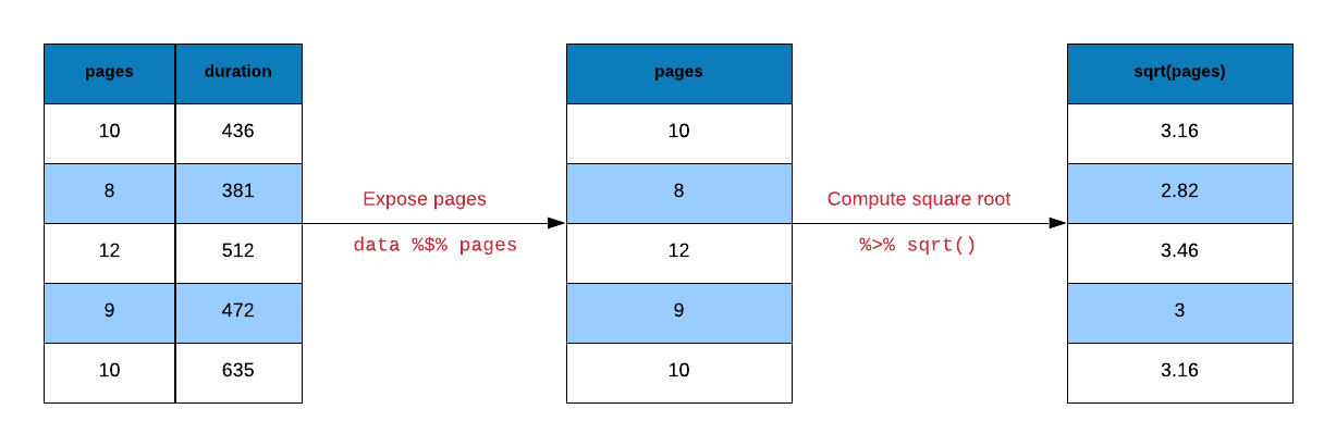ompute the square root
• assign the first few observations to y

Let us reproduce y using pipes.

# extract the n_pages column and assign it to y
y <-
  ecom_mini |>
  pull(n_pages)

# compute the square root of y and assign it back to y
y <- sqrt(y)

Another way to compute the square root of y is shown below.

y <-
  ecom_mini |>
  pull(n_pages) |>
  sqrt()

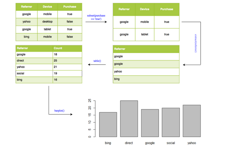
6.6 Visualization

Let us look at a data visualization example. We will create a bar plot to visualize the frequency of different referrer types that drove purchasers to the website. Let us look at the steps involved in creating the bar plot:

• extract rows where purchase is TRUE
• select/expose referrer column
• tabulate referrer data using table()
• use the tabulated data to create bar plot using barplot()

barplot(table(subset(ecom, purchase)$referrer))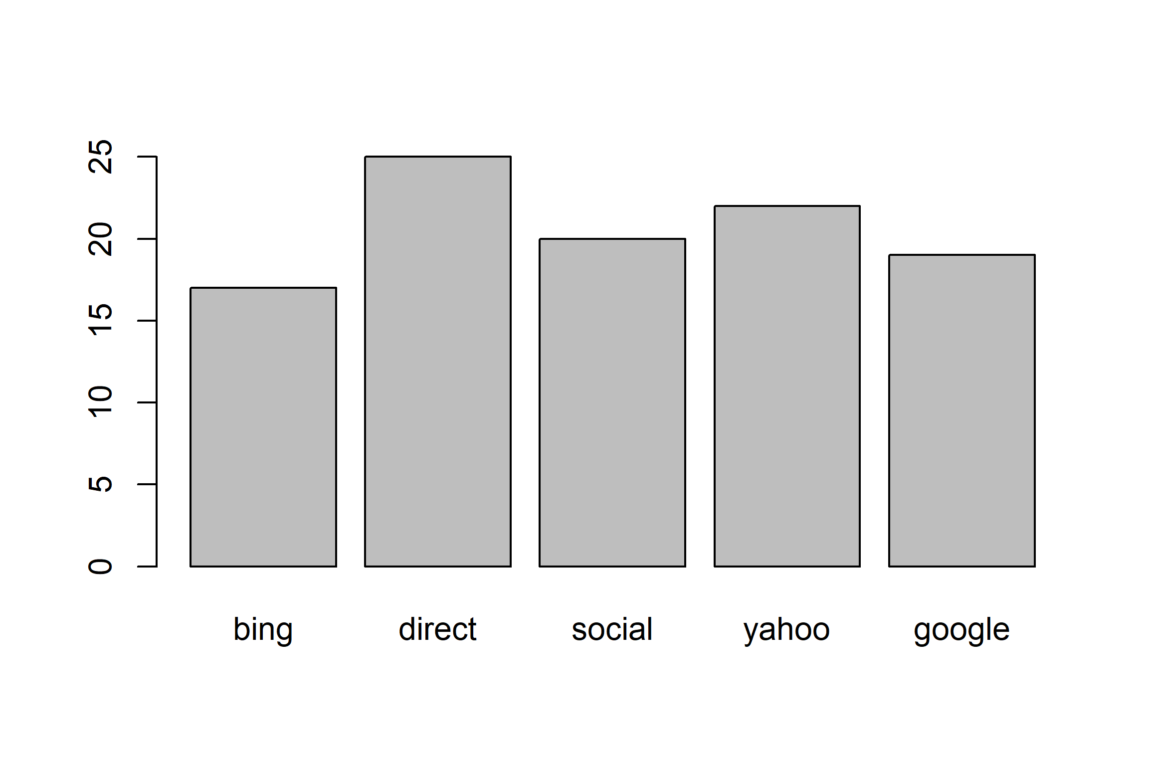

6.6.1 Using pipe

ecom |>
  subset(purchase) |>
  pull('referrer') |>
  table() |>
  barplot()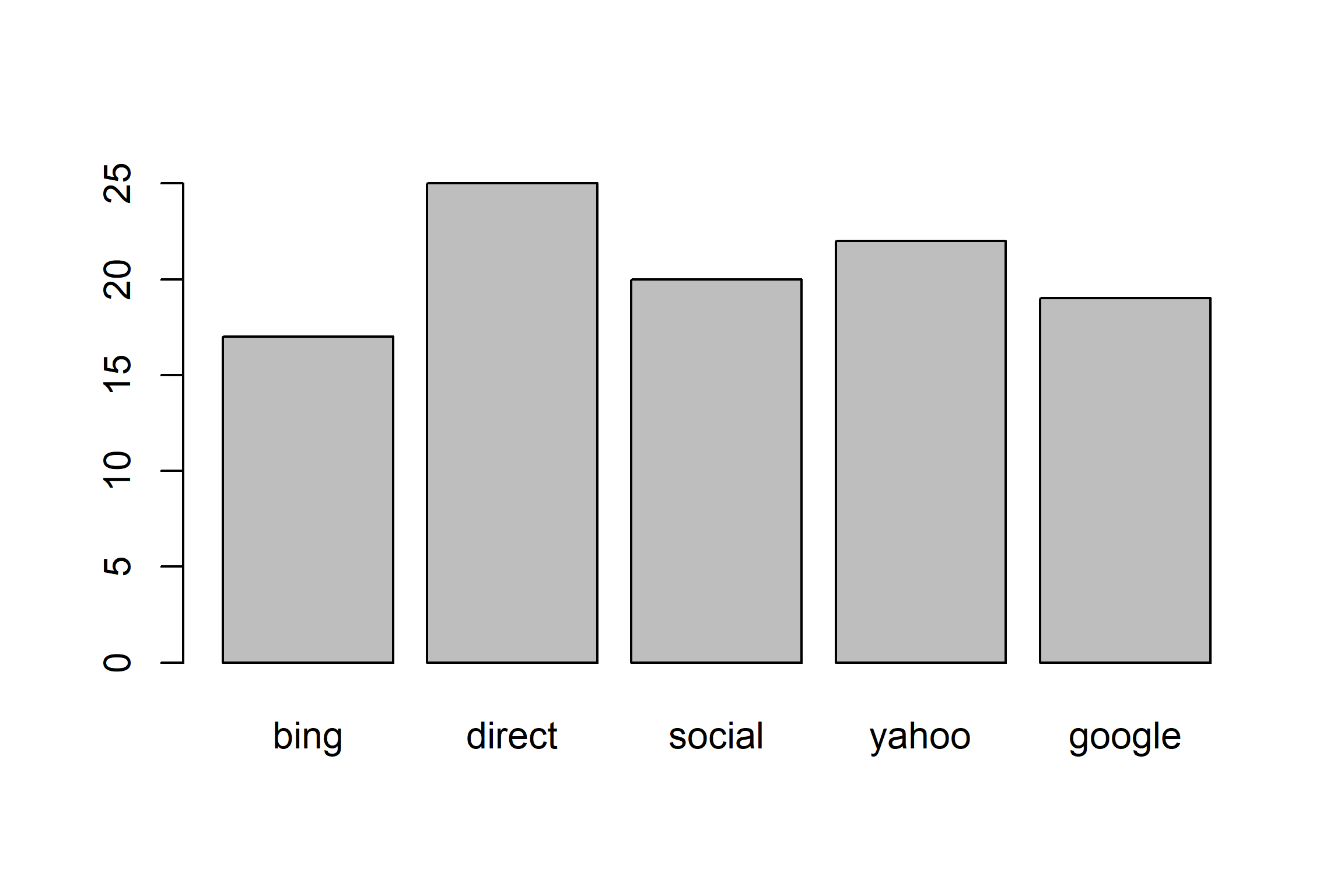

6.7 Correlation

Correlation is a statistical measure that indicates the extent to which two or more variables fluctuate together. In R, correlation is computed using cor(). Let us look at the correlation between the number of pages browsed and time spent on the site for visitors who purchased some product. Below are the steps for computing correlation:

• extract rows where purchase is TRUE
• select/expose n_pages and duration columns
• use cor() to compute the correlation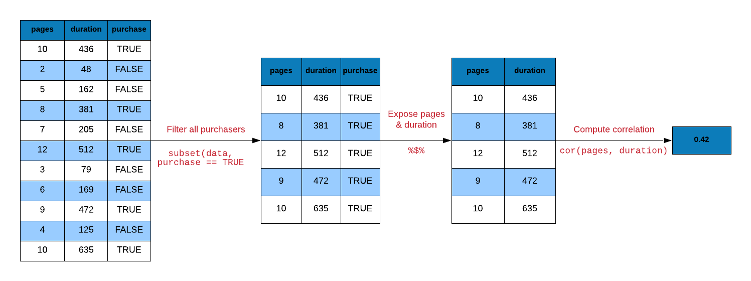

# without pipe
ecom1 <- subset(ecom, purchase)
cor(ecom1$n_pages, ecom1$duration)

[1] 0.4290905

# with pipe
ecom |>
  filter(purchase) |>
  summarise(cor = cor(n_pages, duration))

# A tibble: 1 × 1
    cor
  <dbl>
1 0.429

6.8 Regression

Let us look at a regression example. We regress time spent on the site on number of pages visited. Below are the steps involved in running the regression:

• use duration and n_pages columns from ecom data
• pass the above data to lm()
• pass the output from lm() to summary()

summary(lm(duration ~ n_pages, data = ecom))

Call:
lm(formula = duration ~ n_pages, data = ecom)

Residuals:
    Min      1Q  Median      3Q     Max 
-386.45 -213.03  -38.93  179.31  602.55 

Coefficients:
            Estimate Std. Error t value Pr(>|t|)    
(Intercept)  404.803     11.323  35.750  < 2e-16 ***
n_pages       -8.355      1.296  -6.449 1.76e-10 ***
---
Signif. codes:  0 '***' 0.001 '**' 0.01 '*' 0.05 '.' 0.1 ' ' 1

Residual standard error: 263.3 on 998 degrees of freedom
Multiple R-squared:   0.04, Adjusted R-squared:  0.03904 
F-statistic: 41.58 on 1 and 998 DF,  p-value: 1.756e-10

6.8.1 Using pipe

ecom |>
  with(lm(duration ~ n_pages)) |>
  summary()

Call:
lm(formula = duration ~ n_pages)

Residuals:
    Min      1Q  Median      3Q     Max 
-386.45 -213.03  -38.93  179.31  602.55 

Coefficients:
            Estimate Std. Error t value Pr(>|t|)    
(Intercept)  404.803     11.323  35.750  < 2e-16 ***
n_pages       -8.355      1.296  -6.449 1.76e-10 ***
---
Signif. codes:  0 '***' 0.001 '**' 0.01 '*' 0.05 '.' 0.1 ' ' 1

Residual standard error: 263.3 on 998 degrees of freedom
Multiple R-squared:   0.04, Adjusted R-squared:  0.03904 
F-statistic: 41.58 on 1 and 998 DF,  p-value: 1.756e-10

6.9 String Manipulation

We want to extract the first name (jovial) from the below email id and convert it to upper case. Below are the steps to achieve this:

• split the email id using the pattern @ using str_split()
• extract the first element of the resulting list and the first element of the character vector using pluck()
• extract the first six characters using str_sub()
• convert to upper case using str_to_upper()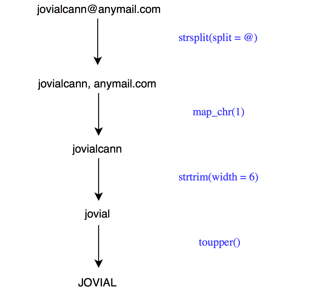

email <- 'jovialcann@anymail.com'

# without pipe
str_to_upper(str_sub(str_split(email, '@')[[1]][1], start = 1, end = 6))

[1] "JOVIAL"

# with pipe
email |>
  str_split(pattern = '@') |>
  pluck(1, 1) |>
  str_sub(start = 1, end = 6) |>
  str_to_upper()

[1] "JOVIAL"

Another method that uses map_chr() from the purrr package.

email |>
  str_split(pattern = '@') |>
  map_chr(1) |>
  str_sub(start = 1, end = 6) |>
  str_to_upper()

[1] "JOVIAL"

6.10 Data Extraction

Let us turn our attention towards data extraction. dplyr and purrr provide pull() and pluck() as readable alternatives to $, [ and [[:

• pull() extracts a column as a vector (like $)
• pluck() extracts an element from a list or vector (like [[)

6.10.1 Extract Column

To extract a specific column using the column name, we mention the name of the column in single/double quotes within [ or [[. In case of $, we do not use quotes.

# base 
ecom_mini['n_pages']

# A tibble: 10 × 1
   n_pages
     <dbl>
 1      18
 2       1
 3      14
 4      17
 5      18
 6      15
 7      20
 8      20
 9       1
10      18

# tidyverse
select(ecom_mini, n_pages)

# A tibble: 10 × 1
   n_pages
     <dbl>
 1      18
 2       1
 3      14
 4      17
 5      18
 6      15
 7      20
 8      20
 9       1
10      18

We can extract columns using their index position. Keep in mind that index position starts from 1 in R. In the below example, we show how to extract n_pages column but instead of using the column name, we use the column position.

# base 
ecom_mini[2]

# A tibble: 10 × 1
   n_pages
     <dbl>
 1      18
 2       1
 3      14
 4      17
 5      18
 6      15
 7      20
 8      20
 9       1
10      18

# tidyverse
select(ecom_mini, 2)

# A tibble: 10 × 1
   n_pages
     <dbl>
 1      18
 2       1
 3      14
 4      17
 5      18
 6      15
 7      20
 8      20
 9       1
10      18

One important differentiator between [ and [[ is that [[ will return an atomic vector and not a data.frame. $ will also return an atomic vector. In the tidyverse, we use pull() in place of $.

# base 
ecom_mini$n_pages

 [1] 18  1 14 17 18 15 20 20  1 18

# tidyverse
pull(ecom_mini, n_pages)

 [1] 18  1 14 17 18 15 20 20  1 18

6.10.2 Extract List Element

Let us convert ecom_mini into a list using as.list() as shown below:

ecom_list <- as.list(ecom_mini)

To extract elements of a list, we use pluck(). It is the tidyverse alternative for [[.

# base 
ecom_list[['n_pages']]

 [1] 18  1 14 17 18 15 20 20  1 18

# tidyverse
pluck(ecom_list, 'n_pages')

 [1] 18  1 14 17 18 15 20 20  1 18

# base 
ecom_list[[1]]

 [1] google google direct social bing   yahoo  bing   social google yahoo 
Levels: bing direct social yahoo google

# tidyverse
pluck(ecom_list, 1)

 [1] google google direct social bing   yahoo  bing   social google yahoo 
Levels: bing direct social yahoo google

We can extract the elements of a list by name using pluck() as well.

# base 
ecom_list$n_pages

 [1] 18  1 14 17 18 15 20 20  1 18

# tidyverse
pluck(ecom_list, "n_pages")

 [1] 18  1 14 17 18 15 20 20  1 18

6.11 Arithmetic Operations

magrittr offer alternatives for arithemtic operations as well. We will look at a few examples below.

• add()
• subtract()
• multiply_by()
• multiply_by_matrix()
• divide_by()
• divide_by_int()
• mod()
• raise_to_power()

6.11.1 Addition

1:10 + 1

 [1]  2  3  4  5  6  7  8  9 10 11

add(1:10, 1)

 [1]  2  3  4  5  6  7  8  9 10 11

`+`(1:10, 1)

 [1]  2  3  4  5  6  7  8  9 10 11

6.11.2 Multiplication

1:10 * 3

 [1]  3  6  9 12 15 18 21 24 27 30

multiply_by(1:10, 3)

 [1]  3  6  9 12 15 18 21 24 27 30

`*`(1:10, 3)

 [1]  3  6  9 12 15 18 21 24 27 30

6.11.3 Division

1:10 / 2

 [1] 0.5 1.0 1.5 2.0 2.5 3.0 3.5 4.0 4.5 5.0

divide_by(1:10, 2)

 [1] 0.5 1.0 1.5 2.0 2.5 3.0 3.5 4.0 4.5 5.0

`/`(1:10, 2)

 [1] 0.5 1.0 1.5 2.0 2.5 3.0 3.5 4.0 4.5 5.0

6.11.4 Power

1:10 ^ 2

  [1]   1   2   3   4   5   6   7   8   9  10  11  12  13  14  15  16  17  18
 [19]  19  20  21  22  23  24  25  26  27  28  29  30  31  32  33  34  35  36
 [37]  37  38  39  40  41  42  43  44  45  46  47  48  49  50  51  52  53  54
 [55]  55  56  57  58  59  60  61  62  63  64  65  66  67  68  69  70  71  72
 [73]  73  74  75  76  77  78  79  80  81  82  83  84  85  86  87  88  89  90
 [91]  91  92  93  94  95  96  97  98  99 100

raise_to_power(1:10, 2)

 [1]   1   4   9  16  25  36  49  64  81 100

`^`(1:10, 2)

 [1]   1   4   9  16  25  36  49  64  81 100

6.12 Logical Operators

There are alternatives for logical operators as well. We will look at a few examples below.

• and()
• or()
• equals()
• not()
• is_greater_than()
• is_weakly_greater_than()
• is_less_than()
• is_weakly_less_than()

6.12.1 Greater Than

1:10 > 5

 [1] FALSE FALSE FALSE FALSE FALSE  TRUE  TRUE  TRUE  TRUE  TRUE

is_greater_than(1:10, 5)

 [1] FALSE FALSE FALSE FALSE FALSE  TRUE  TRUE  TRUE  TRUE  TRUE

`>`(1:10, 5)

 [1] FALSE FALSE FALSE FALSE FALSE  TRUE  TRUE  TRUE  TRUE  TRUE

6.12.2 Weakly Greater Than

1:10 >= 5

 [1] FALSE FALSE FALSE FALSE  TRUE  TRUE  TRUE  TRUE  TRUE  TRUE

is_weakly_greater_than(1:10, 5)

 [1] FALSE FALSE FALSE FALSE  TRUE  TRUE  TRUE  TRUE  TRUE  TRUE

`>=`(1:10, 5)

 [1] FALSE FALSE FALSE FALSE  TRUE  TRUE  TRUE  TRUE  TRUE  TRUE