14  Categorical Data Fundamentals

15 Categorical Data Fundamentals

NoteContinued in part B

This chapter was split for readability. Reordering, recoding, lumping and visualization continue in @forcats-manipulation.

This chapter is the first of two on categorical data. Here we cover what factors are, how R stores them, frequency tabulation and base R pitfalls. @forcats-manipulation continues with reordering, recoding, lumping and ggplot2 visualization.

15.1 Introduction

Handling categorical/qualitative data is integral to data analysis. Almost every data science project involves working with categorical data and students should know how to store, summarize, visualize & manipulate such data. Working with categorical data is different from working with numbers or text. In this chapter, we will understand categorical data and explore the rich set of functions (built-in & through packages) provided by R for working with such data. The word categorical is used interchangeably with qualitative.

15.1.1 Data Types

Before we begin our deep dive on categorical data, let us get a quick overview of different data types.

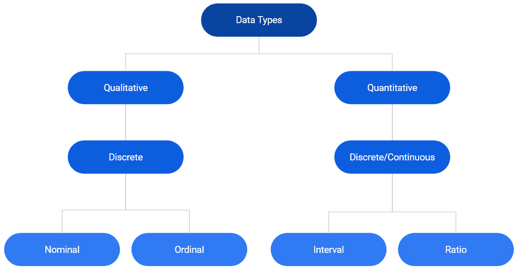
In the chart above, we can see that data can be primarily classified into qualitative or quantitative. Qualitative data consists of labels or names. Quantitative data, on the other hand, consists of numbers and indicate how much or how many. This brings us to the next level of classification:

• discrete
• continuous

In the chart, we can observe that qualitative data is always discrete where as quantitative data may be discrete or continuous. Qualitative data is further classified into

• nominal
• ordinal

First, we will understand discrete and continuous data, and then proceed to explore nominal and ordinal data.

Discrete Data

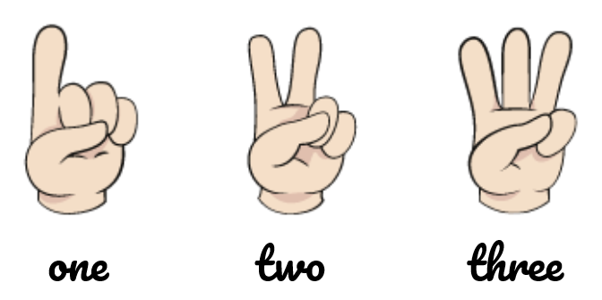
Discrete data arises in situations where counting is involved. It can take on only a finite number of values and cannot be divided into smaller parts. For example, let us consider the number of students in a class. We can have 5 0r 10 students but not 5.5 students (we can’t have half a student).

Continuous Data

Continuous data arises in situations where measuring is involved. It can take any numeric value in a specified range and can be divided into smaller parts and still have meaning. Examples include money, temperature, length, volume etc.

15.1.2 Categorical Data

Since our interest is in categorical data, we will spend more time understanding the different types of categorical data through various examples. Let us begin by formally defining categorical data:

• it is always discrete
• it may be divided into groups
• consists of names or labels
• takes on limited & fixed number of possible values
• arises in situation when counting is involved
• analysis generally involves the use of data tables

15.1.3 Dichotomous

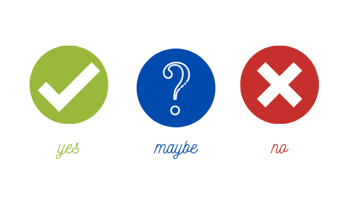
A categorical variable that can take on exactly two values is termed as binary or dichotomous variable.

15.1.4 Polychotomous

Categorical variables with more than two possible values are called polychotomous variables.

15.1.5 Ordinal

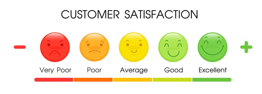
In ordinal data, the categories can be ordered or ranked. Examples include

• socio-economic status
• education level
• income level
• satisfaction rating

While we can rank the categories, we cannot assign a value to them. For example, in satisfaction ranking, we cannot say that like is twice as positive as dislike i.e. we are unable to say how much they differ from each other. While the order or rank of data is meaningful, the difference between two pieces of data cannot be measured/determined or are meaningless. Ordinal data provide information about relative comparisons, but not the magnitude of the differences.

15.1.6 Nominal

Nominal data do not have an intrinsic order and cannot be ordered or measured. Examples include

• blood group
• gender
• religion
• color

Categorical data are sometimes coded with numbers, with those numbers replacing names. Although such numbers might appear to be quantitative, they are actually categorical data. When they do take numerical values, those numbers do not have any mathematical meaning. Examples include months expressed in numbers.

15.1.7 Summary

• Data can be qualitative or quantitative.
• Qualitative data is always discrete.
• Dichotomous data consists of only 2 groups/levels.
• Polychotomous data consists of more than 2 groups/levels.
• Nominal data do not have an intrinsic order.
• In ordinal data
  • categories can be ordered or ranked
  • the difference between the categories cannot be determined

15.1.8 Your Turn…

1. State whether the following are quantitative or qualitative

• Age
• Gender
• Annual Sales
• Weight
• Education Level
• Vehicle Type
• Height
• Ice Cream Flavor
• Job/Work Experience
• Blood Group
• Color
• Mode of Payment

2. State whether the following are dichotomous or polychotomous

• Heads / Tails
• Blood Group
• Transportation Mode
• Rich / Poor
• Democrat / Republican
• Education Level
• Gender
• Pass / Fail
• Yes / No
• Positive / Negative

3. State whether the following are nominal or ordinal

• STD Codes
• Prepaid / Postpaid
• Hotel Ratings
• Smart Phone Brands
• Student Grades
• Cellular Operator
• ISPs (Internet Service Providers)
• Occupation
• Bank Account Number
• Class of Travel
• Military Rank

15.2 Case Study

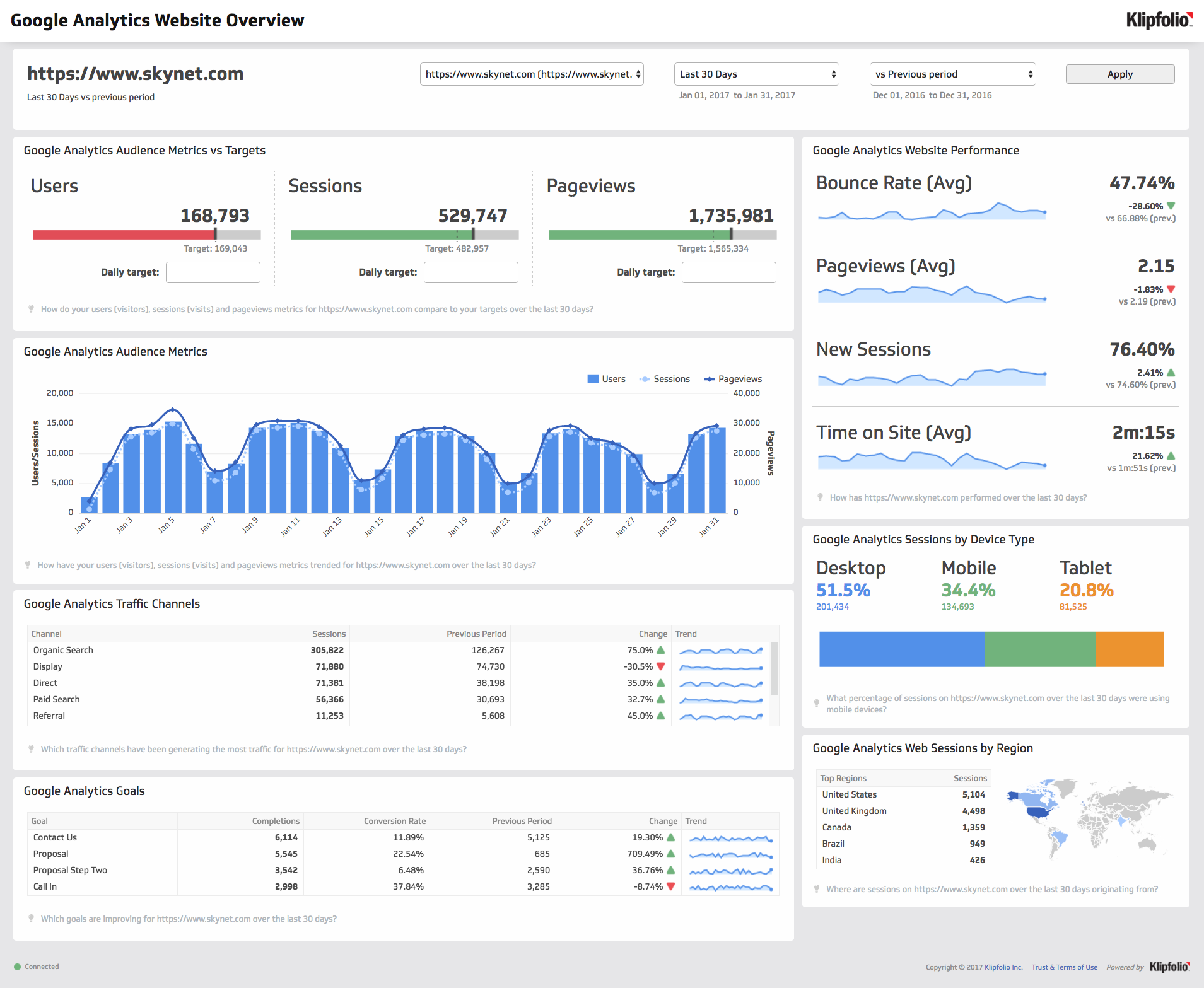
As is the practice, throughout this chapter, we will work on a case study related to an e-commerce firm. As most of you would already be aware, a lot of data is captured when you go on the internet by the websites you browse as well as by third party cookies. Data collected is then used to display ads as well as to feed to recommendation algorithms.

The data used in the case study represents the basic information that is captured when users visit any website. It closely resembles real world data for an e-commerce store. We will try to generate insights about the visitors to be used by an imaginary marketing team for better targeting and promotion. The case study data set can be imported using the RStudio IDE or R code.

15.2.1 Data

The data set is available in both CSV & RDS formats.

CSV

If you want to specify the data types while reading the data, use the readr package. We have explored how to import data into R in a previous chapter. We will read a subset of columns from the data set (it has 20 columns) which will cover both nominal and ordinal data types. To import the data, we will use the read_csv() function. The first input is the name of the data set, analytics.csv. Ensure that the name is enclosed in single/double quotes.

read_csv("analytics_raw.csv", 
         col_types = cols_only(device = col_factor(levels = c("Desktop", "Tablet", "Mobile")), 
                               gender = col_factor(levels = c("female", "male", "NA")), 
                               user_rating = col_factor(levels = c("1", "2", "3", "4", "5"),
                                                        ordered = TRUE)))

# A tibble: 244,398 × 3
   device  gender user_rating
   <fct>   <fct>  <ord>      
 1 Desktop female 4          
 2 Mobile  NA     5          
 3 Desktop NA     4          
 4 Desktop NA     5          
 5 Desktop NA     4          
 6 Mobile  NA     4          
 7 Desktop NA     4          
 8 Desktop NA     4          
 9 Desktop female 5          
10 Desktop NA     4          
# ℹ 244,388 more rows

Since we are specifying the column data types while importing the data, we will use the col_types argument to list out the data types. As we are reading in a subset of the columns and not all of them, we will use the cols_only() function indicating that only the columns specified must be read in and not all of them.

Categorical data and the levels/groups are specified using the col_factor() function. Use the levels argument to specify the levels/groups and the ordered argument to indicate if the data is ordinal. By default, it is set to FALSE, change this to TRUE if the column is ordinal.

RDS

The .rds file can be read using readRDS().

data <- readRDS('analytics.rds')
head(data)

# A tibble: 6 × 19
  device  os       browser user_type channel gender frequency recency page_depth
  <fct>   <fct>    <fct>   <fct>     <fct>   <fct>      <dbl>   <dbl>      <dbl>
1 Desktop Windows  Chrome  New Visi… Organi… female         1       0          1
2 Mobile  iOS      Safari  Returnin… Organi… <NA>           3       1          1
3 Desktop Chrome … Chrome  New Visi… Direct  <NA>           1       0          5
4 Desktop Macinto… Chrome  Returnin… Organi… <NA>           2       0          1
5 Desktop Macinto… Chrome  Returnin… Referr… <NA>           5       8          1
6 Mobile  Android  Chrome  New Visi… Organi… <NA>           1       0          5
# ℹ 10 more variables: hour_of_day <chr>, age <dbl>, duration <dbl>,
#   landing_page <fct>, exit_page <fct>, country <fct>, quantity <dbl>,
#   revenue <dbl>, purchase_flag <lgl>, user_rating <dbl>

15.2.2 Data Dictionary

Column	Description
device	Device used to browse the website
os	Operating system of the device
browser	Browser used to visit the website
user_type	New or returning visitor
channel	Source of traffic
gender	Gender of the visitor
frequency	Count of visits to the website
recency	Number of days since last visit
page_depth	Number of website pages browsed
hour_of_day	Hour of day
age	Age of the visitor
duration	Time spent on the website (in seconds)
landing_page	Page on which visitor landed
exit_page	Page on which visitor exited
country	Country of origin
city	City of the visitor
quantity	Number of units purchased
revenue	Total revenue
purchase_flag	Whether the visitor checked out?
user_rating	Website UI rating given by visitor

15.3 Factors

In this very important section, we will learn how R

• stores categorical data
• checks if given data is categorical
• converts other data types to factor
• handles missing values in categorical data
• specifies the orders of the categories/levels
• stores ordinal data

15.3.1 Introduction

In R, categorical data is stored as factor. Before we explore the factor family of functions, let us generate the sample data we will use in this module. We will generate the device column from the case study data set using the sample() function. We provide the following inputs to generate the data:

• values from which the data must be generated
• the size of the sample
• indicate if the values must be repeated (TRUE/FALSE)

device <- sample(c("Desktop", "Mobile", "Tablet"), size = 25, replace = TRUE)
device

 [1] "Desktop" "Desktop" "Mobile"  "Mobile"  "Desktop" "Mobile"  "Tablet" 
 [8] "Desktop" "Mobile"  "Tablet"  "Mobile"  "Desktop" "Tablet"  "Mobile" 
[15] "Desktop" "Mobile"  "Mobile"  "Mobile"  "Mobile"  "Desktop" "Desktop"
[22] "Tablet"  "Mobile"  "Tablet"  "Mobile" 

15.3.2 Membership Testing

Great! We have successfully generated the sample data and along the way learnt a new R function for sampling. First, let us check if the sample is a factor using the membership function is.factor().

is.factor(device)

[1] FALSE

Membership testing functions always have the prefix is_ and return only logical values. If the object is a member of the specified class, they return TRUE else FALSE. Since our sample data is not stored as a factor, R has returned FALSE.

15.3.3 Coercion

Let us try to coerce it into factor using the coercion function as.factor().

as.factor(device)

 [1] Desktop Desktop Mobile  Mobile  Desktop Mobile  Tablet  Desktop Mobile 
[10] Tablet  Mobile  Desktop Tablet  Mobile  Desktop Mobile  Mobile  Mobile 
[19] Mobile  Desktop Desktop Tablet  Mobile  Tablet  Mobile 
Levels: Desktop Mobile Tablet

Do you spot any difference in the output? In the last line, it displays the levels or categories of the variable. Don’t worry if you didn’t spot it. We are just getting started and you will pick it up by the end of this section. Another function that can be used to coerce data into factor is as_factor() from the forcats package.

as_factor(device)

 [1] Desktop Desktop Mobile  Mobile  Desktop Mobile  Tablet  Desktop Mobile 
[10] Tablet  Mobile  Desktop Tablet  Mobile  Desktop Mobile  Mobile  Mobile 
[19] Mobile  Desktop Desktop Tablet  Mobile  Tablet  Mobile 
Levels: Desktop Mobile Tablet

Did you notice any difference between these two functions? Focus on the last line of the output where the levels are displayed. Now observe the order of the levels. as.factor() displays levels in the alphabetical order whereas as_factor() displays them in order of appearance in the data. Mobile, followed by Tablet, and then Desktop. If you look at the data, they appear in the same order.

15.3.4 Factor Function

If you want finer control while creating factors, use the factor() function. as.factor() should suffice in most cases but use factor() when you want to:

• specify levels
• modify labels
• include NA as a level/category
• create ordered factors
• specify order of levels

The first input is a vector, usually a numeric or character vector with a small number of unique values. In our example, it is a character vector of length 25 (i.e. 25 values) but 3 unique values.

factor(device)

 [1] Desktop Desktop Mobile  Mobile  Desktop Mobile  Tablet  Desktop Mobile 
[10] Tablet  Mobile  Desktop Tablet  Mobile  Desktop Mobile  Mobile  Mobile 
[19] Mobile  Desktop Desktop Tablet  Mobile  Tablet  Mobile 
Levels: Desktop Mobile Tablet

If you want to specify the levels or categories, use the levels argument.

factor(device, levels = c("Desktop", "Mobile", "Tablet"))

 [1] Desktop Desktop Mobile  Mobile  Desktop Mobile  Tablet  Desktop Mobile 
[10] Tablet  Mobile  Desktop Tablet  Mobile  Desktop Mobile  Mobile  Mobile 
[19] Mobile  Desktop Desktop Tablet  Mobile  Tablet  Mobile 
Levels: Desktop Mobile Tablet

Levels not specified will be replaced by NA. Let us specify only Desktop and Mobile as the levels in the device column and see what happens.

factor(device, levels = c("Desktop", "Mobile"))

 [1] Desktop Desktop Mobile  Mobile  Desktop Mobile  <NA>    Desktop Mobile 
[10] <NA>    Mobile  Desktop <NA>    Mobile  Desktop Mobile  Mobile  Mobile 
[19] Mobile  Desktop Desktop <NA>    Mobile  <NA>    Mobile 
Levels: Desktop Mobile

As you can see, Tablet has been replaced by NA.

15.3.5 Modify Labels

You can change the labels of the levels using the labels argument. The labels must be in the same order as the levels. We will modify the labels to Desk, Mob & Tab for Desktop, Mobile & Tablet respectively.

factor(device, 
       levels = c("Desktop", "Mobile", "Tablet"),
       labels = c("Desk", "Mob", "Tab"))

 [1] Desk Desk Mob  Mob  Desk Mob  Tab  Desk Mob  Tab  Mob  Desk Tab  Mob  Desk
[16] Mob  Mob  Mob  Mob  Desk Desk Tab  Mob  Tab  Mob 
Levels: Desk Mob Tab

You can see that not only the values but the levels are also modified.

15.3.6 Missing Values

Let us regenerate the device column but include some missing values (NA) deliberately to see how factor() handles them.

# sample with missing values
device <- sample(c("Desktop", "Mobile", "Tablet", NA), size = 25, replace = TRUE)
device

 [1] "Tablet"  "Tablet"  NA        "Mobile"  "Tablet"  "Mobile"  NA       
 [8] NA        "Tablet"  "Tablet"  "Mobile"  "Mobile"  NA        "Tablet" 
[15] "Desktop" "Tablet"  "Mobile"  NA        "Tablet"  NA        "Desktop"
[22] "Mobile"  NA        "Desktop" "Mobile" 

# store as categorical data
factor(device)

 [1] Tablet  Tablet  <NA>    Mobile  Tablet  Mobile  <NA>    <NA>    Tablet 
[10] Tablet  Mobile  Mobile  <NA>    Tablet  Desktop Tablet  Mobile  <NA>   
[19] Tablet  <NA>    Desktop Mobile  <NA>    Desktop Mobile 
Levels: Desktop Mobile Tablet

NA is not shown as one of the levels. Why does this happen? By default, it will ignore them. If you look at the arguments of the factor() function, the exclude argument is set to NA by default i.e. NA is excluded automatically. What should we do to ensure that NA is also treated as a level? In order to treat NA as a level, set the exclude argument to NULL.

factor(device, exclude = NULL)

 [1] Tablet  Tablet  <NA>    Mobile  Tablet  Mobile  <NA>    <NA>    Tablet 
[10] Tablet  Mobile  Mobile  <NA>    Tablet  Desktop Tablet  Mobile  <NA>   
[19] Tablet  <NA>    Desktop Mobile  <NA>    Desktop Mobile 
Levels: Desktop Mobile Tablet <NA>

As you can see, NA is displayed as one of the levels in the data.

15.3.7 Ordered Factors

So far, we have been looking at nominal data. Let us now explore how R handles ordered data. We will generate a new data set of satisfaction ratings to use in this section. Satisfaction ratings are widely used to measure a customer’s satisfaction with an organization, service or a product.

rating <- sample(c("Dislike", "Neutral", "Like"), size = 25, replace = TRUE)
rating

 [1] "Neutral" "Neutral" "Dislike" "Dislike" "Like"    "Dislike" "Neutral"
 [8] "Dislike" "Like"    "Neutral" "Dislike" "Dislike" "Neutral" "Dislike"
[15] "Dislike" "Dislike" "Neutral" "Neutral" "Neutral" "Neutral" "Neutral"
[22] "Dislike" "Like"    "Neutral" "Neutral"

It consists of three values Dislike, Neutral & Like in that order. You can see that there is an intrinsic order here. Like is better than neutral which in turn is better than dislike. While we can order them, we can’t quantify the difference between them. We can’t say neutral is so many times better than dislike.

Membership Testing

As we did earlier, let us check if the data is ordered using the membership function is.ordered().

is.ordered(rating)

[1] FALSE

R returns FALSE as the variable rating is not ordered. Let us use as.ordered() to coerce it into an ordered factor.

as.ordered(rating)

 [1] Neutral Neutral Dislike Dislike Like    Dislike Neutral Dislike Like   
[10] Neutral Dislike Dislike Neutral Dislike Dislike Dislike Neutral Neutral
[19] Neutral Neutral Neutral Dislike Like    Neutral Neutral
Levels: Dislike < Like < Neutral

Look at the last line where the levels are displayed. In case of ordered factors, you will see a < between the labels. This is used to indicate the order of the levels. Now rating is both an ordered but the order of the levels is not correct. It should be Dislike < Neutral < Like but is displayed in order of appearance in the data. Let us use the factor() function since we need more control over how the levels are ranked and set the ordered argument to TRUE.

factor(rating, ordered = TRUE)

 [1] Neutral Neutral Dislike Dislike Like    Dislike Neutral Dislike Like   
[10] Neutral Dislike Dislike Neutral Dislike Dislike Dislike Neutral Neutral
[19] Neutral Neutral Neutral Dislike Like    Neutral Neutral
Levels: Dislike < Like < Neutral

The ranking of the levels has not changed and is still the same. Why is this happening? If you observe carefully, the ranking follows the alphabetical order (Desktop, Mobile, Table). The factor() function uses the same order for the levels.

15.3.8 Modify Order of Levels

To change the order/ranking of the levels, we need to specify it using the levels argument. Let us do that in the next example.

factor(rating, levels = c("Dislike", "Neutral", "Like"), ordered = TRUE)

 [1] Neutral Neutral Dislike Dislike Like    Dislike Neutral Dislike Like   
[10] Neutral Dislike Dislike Neutral Dislike Dislike Dislike Neutral Neutral
[19] Neutral Neutral Neutral Dislike Like    Neutral Neutral
Levels: Dislike < Neutral < Like

Now, you can see that the levels are ranked correctly. The ordered() function can also be used to create ordered factors. Let us recreate the previous example using the ordered() function.

ordered(rating, levels = c("Dislike", "Neutral", "Like"))

 [1] Neutral Neutral Dislike Dislike Like    Dislike Neutral Dislike Like   
[10] Neutral Dislike Dislike Neutral Dislike Dislike Dislike Neutral Neutral
[19] Neutral Neutral Neutral Dislike Like    Neutral Neutral
Levels: Dislike < Neutral < Like

You can specify levels, modify labels and handle missing values using the ordered() function as well.

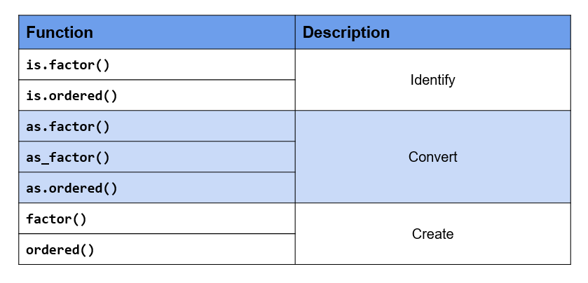
15.3.9 Key Functions

15.3.10 Summary

• R uses factor to handle categorical data.
• Use as.factor() or as_factor() to coerce other data types to factor.
• Use is.factor() or is.ordered() to identify factor & ordered factor respectively.
• Use factor() to
  • specify labels
  • modify labels
  • handle missing data
  • create ordered factors
  • specify order of levels
• Use ordered() to create ordered factors.

15.3.11 Your Turn…

Use analytics_raw.rds data set to answer the below questions.

1. Check whether the below variables are factor

   • device
   • page_depth
   • landing_page

2. Coerce the following variables to type factor

   • device
   • os
   • browser
   • user_type
   • channel
   • gender
   • landing_page
   • exit_page
   • city
   • country
   • user_type

3. Use only the following levels in the gender column:

   • male
   • female

4. Include NA as a level in the gender column.

5. Change label of NA to missing in the gender column.

6. Change the labels of the levels in user_type column to

   • New
   • Returning

7. Check if the user_rating column is ordered. If not, coerce it to type ordered factor.

15.4 Summarize

15.4.1 Introduction

Categorical data cannot be summarized in the same way as numeric data. It does not make sense to look at range, standard deviation etc. since data consists of a few distinct values only. So how do we summarize such data? We can look at

• count/frequency
• proportion
• cumulative frequency
• cross table
• contingency table etc.

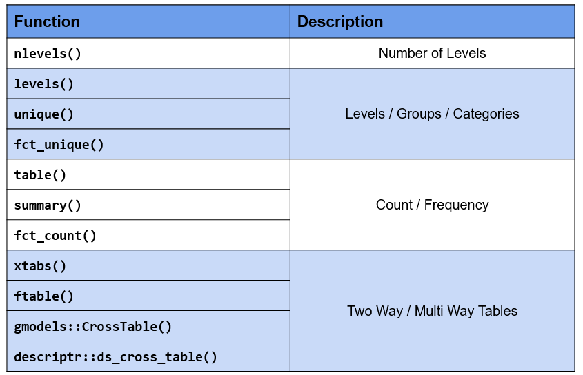
In this section, we will explore the above ways of summarizing categorical data. We will also spend some time learning about tables as you will be using them extensively while working with categorical data. R has many packages for tabulating data and we list and explore all of them in the last section of this chapter.

15.4.2 Number of Categories

From our case study, we want to know the number of devices used to browse the website, the name of the devices and the proportion of traffic they drive to our website. Let us begin with the number of devices. To view the number of groups/categories in a categorical variable, use nlevels().

nlevels(data$device)

[1] 3

There are 3 categories of devices used by the visitors to browse the website. This can also be used for data sanitization i.e. as an analyst you know that there are only 3 valid categories of device into which any visitor can be classified into. If you see more than 3 categories, you might want to check if there are any issues in data collection or processing. Now that we know there are 3 categories of devices, let us check if they are valid. The levels() function will return the labels of the groups.

15.4.3 Category Names

Knowing the number of levels is useful but not sufficient. levels() is one of the most useful functions when it comes to dealing with categorical data.

levels(data$device)

[1] "Desktop" "Mobile"  "Tablet" 

Other functions that you can use include unique() and fct_unique(). Both these functions will return the unique names/labels along with the levels while levels() returns the labels of the levels.

unique(data$device)

[1] Desktop Mobile  Tablet 
Levels: Desktop Mobile Tablet

fct_unique(data$device)

[1] Desktop Mobile  Tablet 
Levels: Desktop Mobile Tablet

15.4.4 Names & Counts

So we have checked the number of devices and their names. Let us now examine their distribution i.e. count/frequency. table() and summary() will display the levels and their counts while fct_count() will return a tibble with 2 columns (level & count). It is extremely useful for further data processing or visualization (using ggplot2).

table(data$device)

Desktop  Mobile  Tablet 
 177282   63482    3634 

fct_count(data$device)

# A tibble: 3 × 2
  f            n
  <fct>    <int>
1 Desktop 177282
2 Mobile   63482
3 Tablet    3634

summary(data$device)

Desktop  Mobile  Tablet 
 177282   63482    3634 

15.4.5 Tables

In the previous section, we used the table() function to tabulate categorical data. We will recreate the tabulation for device and store it in a new variable tab.

tab <- table(data$device)
tab

Desktop  Mobile  Tablet 
 177282   63482    3634 

What does this function return? It is not a vector, list, data.frame or matrix. Let us use the class() function to check the class of the object returned by table(). It returns an object of the class table. This is a new type of object. Let us spend some time understanding tables as they are useful for organizing and summarizing categorical data. table is also the most used object when it comes to dealing with categorical data.

The table() function returns the counts of the categories but let us say we want to view the proportion or percentage instead of counts i.e. the proportion or percentage of traffic driven to our website by the different devices. The proportions() or prop.table() function comes in handy in such cases. It takes a table object as input (tab in our case).

prop.table(tab)

   Desktop     Mobile     Tablet 
0.72538237 0.25974844 0.01486919 

proportions(tab)

   Desktop     Mobile     Tablet 
0.72538237 0.25974844 0.01486919 

To get the percentages, multiply the output by 100. Use the round() function to round the decimal places according to your requirements.

proportions(tab) * 100

  Desktop    Mobile    Tablet 
72.538237 25.974844  1.486919 

round(proportions(tab) * 100, 2)

Desktop  Mobile  Tablet 
  72.54   25.97    1.49 

So far, we have used table() to tabulate a single categorical variable. It can be used for a lot more than just tabulating data. We can examine the relationship between two categorical variables as well as create multidimensional tables. Let us look at the relationship between gender and device in our case study. Does gender affect the type of device used? To answer this, we will create a two way or cross table. In the table() function, we can specify multiple variables by separating them with a comma.

tab2 <- table(data$gender, data$device)
tab2

        
         Desktop Mobile Tablet
  female   32803   7268    494
  male     46418  14503    696
  <NA>     98061  41711   2444

Keep in mind that the order of the variables matter. Rows represent the first variable while column represents the second.

table(data$device, data$gender)

         
          female  male  <NA>
  Desktop  32803 46418 98061
  Mobile    7268 14503 41711
  Tablet     494   696  2444

The proportions() function works with two way tables as well.

proportions(tab2)

        
             Desktop      Mobile      Tablet
  female 0.134219593 0.029738378 0.002021293
  male   0.189927904 0.059341729 0.002847814
  <NA>   0.401234871 0.170668336 0.010000082

proportions(tab2) * 100

        
            Desktop     Mobile     Tablet
  female 13.4219593  2.9738378  0.2021293
  male   18.9927904  5.9341729  0.2847814
  <NA>   40.1234871 17.0668336  1.0000082

We would like to introduce another function at this point of time, margin.table(). What does this function do? It computes the marginal frequencies i.e. the sum of the rows or columns. It takes a table object as input. The margin argument allows us to specify whether we want the sum of rows or columns. 1 indicates rows and 2 indicates columns.

margin.table(tab2, 1) # sum of rows

female   male   <NA> 
 40565  61617 142216 

margin.table(tab2, 2) # sum of columns

Desktop  Mobile  Tablet 
 177282   63482    3634 

If the margin argument is NULL (which it is by default), the function returns the sum of all cells of the table.

margin.table(tab2)

[1] 244398

table() does not display row or column labels. It does display the group labels though. Let us revisit the output from tab2. You can observe that while it includes the group labels, the row and column labels are missing. The output from the dimnames() function shows the group labels of the variables but the row & column labels are absent.

dimnames(tab2)

[[1]]
[1] "female" "male"   NA      

[[2]]
[1] "Desktop" "Mobile"  "Tablet" 

names(tab2)

NULL

names(dimnames(tab2)) 

[1] "" ""

The output from names(dimnames(tab2)) is also empty. Let us add the variable names as the row & column labels to tab2.

names(dimnames(tab2)) <- c("Gender", "Device")
tab2

        Device
Gender   Desktop Mobile Tablet
  female   32803   7268    494
  male     46418  14503    696
  <NA>     98061  41711   2444

Now look at the output from tab2 and you can observe the difference. The same is also visible when we run dimnames(tab2).

dimnames(tab2)

$Gender
[1] "female" "male"   NA      

$Device
[1] "Desktop" "Mobile"  "Tablet" 

To add margin totals to the table, use addmargins(). Like proportions() and margin.table(), it also takes a table object as the input.

addmargins(tab2)

        Device
Gender   Desktop Mobile Tablet    Sum
  female   32803   7268    494  40565
  male     46418  14503    696  61617
  <NA>     98061  41711   2444 142216
  Sum     177282  63482   3634 244398

rowSums() returns the row total while colSums() returns the column total. They are similar to margin.table().

rowSums(tab2)

female   male   <NA> 
 40565  61617 142216 

colSums(tab2)

Desktop  Mobile  Tablet 
 177282   63482    3634 

xtabs() is another way of creating multidimensional tables in R. In comparison to table(), it

• uses formula notation for input
• the data argument ensures variable names are referenced instead of using $ i.e. data$variable
• displays row & column labels by default

tabx <- xtabs(~gender+device, data = data)
tabx

        device
gender   Desktop Mobile Tablet
  female   32803   7268    494
  male     46418  14503    696
  <NA>     98061  41711   2444

The following functions work with xtabs() as well

• proportions()
• margin.table()
• addmargins()

proportions(tabx)

        device
gender       Desktop      Mobile      Tablet
  female 0.134219593 0.029738378 0.002021293
  male   0.189927904 0.059341729 0.002847814
  <NA>   0.401234871 0.170668336 0.010000082

margin.table(tabx, 1)

gender
female   male   <NA> 
 40565  61617 142216 

margin.table(tabx, 2)

device
Desktop  Mobile  Tablet 
 177282   63482    3634 

addmargins(tabx)

        device
gender   Desktop Mobile Tablet    Sum
  female   32803   7268    494  40565
  male     46418  14503    696  61617
  <NA>     98061  41711   2444 142216
  Sum     177282  63482   3634 244398

So far, we have been working with one or two dimensional tables. Both the table() and xtabs() functions are capable of creating multidimensional tables. Keep in mind that multidimensional tables are complex and it becomes increasingly difficult to understand or interpret them.

tab3 <- xtabs(~gender+device+channel, data = data)
tab3

, , channel = (Other)

        device
gender   Desktop Mobile Tablet
  female     786    258      0
  male      1063    507     19
  <NA>      2173   1186     81

, , channel = Affiliates

        device
gender   Desktop Mobile Tablet
  female    1314     60      0
  male      1714    169      0
  <NA>      3518    548     65

, , channel = Direct

        device
gender   Desktop Mobile Tablet
  female    4785    977     59
  male      7010   2381     95
  <NA>     15824   8292    430

, , channel = Display

        device
gender   Desktop Mobile Tablet
  female     123    753    104
  male       210    491     73
  <NA>       554    911    156

, , channel = Organic Search

        device
gender   Desktop Mobile Tablet
  female   17109   4480    282
  male     25016   9563    448
  <NA>     54071  27223   1476

, , channel = Paid Search

        device
gender   Desktop Mobile Tablet
  female     645    230     22
  male       887    478     26
  <NA>      1274    782     51

, , channel = Referral

        device
gender   Desktop Mobile Tablet
  female    7387     74      0
  male      9251    185      0
  <NA>     18052    615     51

, , channel = Social

        device
gender   Desktop Mobile Tablet
  female     654    436     27
  male      1267    729     35
  <NA>      2595   2154    134

ftable stands for flat tables and is useful for printing attractive tables. It makes it easy to read and interpret multidimensional tables. In the next example, we will use ftable() to print the tables we have created in the previous examples and compare the outputs.

ftable(tabx)

       device Desktop Mobile Tablet
gender                             
female          32803   7268    494
male            46418  14503    696
NA              98061  41711   2444

ftable(tab2)

       Device Desktop Mobile Tablet
Gender                             
female          32803   7268    494
male            46418  14503    696
NA              98061  41711   2444

ftable(tab3)

               channel (Other) Affiliates Direct Display Organic Search Paid Search Referral Social
gender device                                                                                      
female Desktop             786       1314   4785     123          17109         645     7387    654
       Mobile              258         60    977     753           4480         230       74    436
       Tablet                0          0     59     104            282          22        0     27
male   Desktop            1063       1714   7010     210          25016         887     9251   1267
       Mobile              507        169   2381     491           9563         478      185    729
       Tablet               19          0     95      73            448          26        0     35
NA     Desktop            2173       3518  15824     554          54071        1274    18052   2595
       Mobile             1186        548   8292     911          27223         782      615   2154
       Tablet               81         65    430     156           1476          51       51    134

By default, missing values (NAs) are excluded from tables. Let us modify the gender data from our case study a bit and see how the table() function deals with missing values. We won’t explicitly specify NA as a level while recreating the gender data.

gen <- as.factor(as.character(data$gender))
table(gen)

gen
female   male 
 40565  61617 

As you can see, table() excludes missing values while tabulating the data. In order to ensure that missing values are also counted, we can use the useNA argument. It can take two values:

• ifany
• always

In the first case, it will show NA as a level and the count only if there are missing values in the data. In the second case, it will always show NA as a level irrespective of whether there are missing values in the data or not.

table(gen, useNA = "ifany")

gen
female   male   <NA> 
 40565  61617 142216 

table(data$device, useNA = "always")

Desktop  Mobile  Tablet    <NA> 
 177282   63482    3634       0 

In this final section on tables, we will learn how to select/access the different parts of a table. We will use [ operator to select rows and columns of a table (it is similar to selecting data from a data.frame). Below are a few examples:

• select first row

tab2[1, ]           

Desktop  Mobile  Tablet 
  32803    7268     494 

• select first column

tab2[, 1]           

female   male   <NA> 
 32803  46418  98061 

• select first two rows

tab2[1:2, ]         

        Device
Gender   Desktop Mobile Tablet
  female   32803   7268    494
  male     46418  14503    696

• select first two columns

tab2[, 1:2]        

        Device
Gender   Desktop Mobile
  female   32803   7268
  male     46418  14503
  <NA>     98061  41711

• select nth row

tab2[2, ]          

Desktop  Mobile  Tablet 
  46418   14503     696 

• select nth column

tab2[, 2]          

female   male   <NA> 
  7268  14503  41711 

• select row by group label

tab2["female", ]   

Desktop  Mobile  Tablet 
  32803    7268     494 

• select column by group label

tab2[, "Mobile"]   

female   male   <NA> 
  7268  14503  41711 

Before we end this section, let us learn how to test if an object is of class table using is.table().

is.table(tab2)

[1] TRUE

Next, we will look at different R packages for two way/contingency tables.

15.4.6 Contingency Table

For cross tables with output similar to SAS or SPSS, use any of the below:

• CrossTable() from the gmodels package
• ds_cross_table() from the descriptr package

gmodels::CrossTable(data$device, data$gender)

 
   Cell Contents
|-------------------------|
|                       N |
| Chi-square contribution |
|           N / Row Total |
|           N / Col Total |
|         N / Table Total |
|-------------------------|

 
Total Observations in Table:  102182 

 
             | data$gender 
 data$device |    female |      male | Row Total | 
-------------|-----------|-----------|-----------|
     Desktop |     32803 |     46418 |     79221 | 
             |    58.228 |    38.334 |           | 
             |     0.414 |     0.586 |     0.775 | 
             |     0.809 |     0.753 |           | 
             |     0.321 |     0.454 |           | 
-------------|-----------|-----------|-----------|
      Mobile |      7268 |     14503 |     21771 | 
             |   218.694 |   143.975 |           | 
             |     0.334 |     0.666 |     0.213 | 
             |     0.179 |     0.235 |           | 
             |     0.071 |     0.142 |           | 
-------------|-----------|-----------|-----------|
      Tablet |       494 |       696 |      1190 | 
             |     0.986 |     0.649 |           | 
             |     0.415 |     0.585 |     0.012 | 
             |     0.012 |     0.011 |           | 
             |     0.005 |     0.007 |           | 
-------------|-----------|-----------|-----------|
Column Total |     40565 |     61617 |    102182 | 
             |     0.397 |     0.603 |           | 
-------------|-----------|-----------|-----------|

 

descriptr::ds_cross_table(data, device, gender)

    Cell Contents
 |---------------|
 |     Frequency |
 |       Percent |
 |       Row Pct |
 |       Col Pct |
 |---------------|

 Total Observations:  244398 

----------------------------------------------------------------------------
|              |                          gender                           |
----------------------------------------------------------------------------
|       device |       female |         male |           NA |    Row Total |
----------------------------------------------------------------------------
|      Desktop |        32803 |        46418 |        98061 |       177282 |
|              |        0.134 |         0.19 |        0.401 |              |
|              |         0.19 |         0.26 |         0.55 |         0.73 |
|              |         0.81 |         0.75 |         0.69 |              |
----------------------------------------------------------------------------
|       Mobile |         7268 |        14503 |        41711 |        63482 |
|              |         0.03 |        0.059 |        0.171 |              |
|              |         0.11 |         0.23 |         0.66 |         0.26 |
|              |         0.18 |         0.24 |         0.29 |              |
----------------------------------------------------------------------------
|       Tablet |          494 |          696 |         2444 |         3634 |
|              |        0.002 |        0.003 |         0.01 |              |
|              |         0.14 |         0.19 |         0.67 |         0.01 |
|              |         0.01 |         0.01 |         0.02 |              |
----------------------------------------------------------------------------
| Column Total |        40565 |        61617 |       142216 |       244398 |
|              |        0.166 |        0.252 |        0.582 |              |
----------------------------------------------------------------------------

We list and explore different R packages for summarizing categorical data in the last section of this chapter.

15.4.7 Key Functions

15.4.8 Your Turn…

1. Display the number of levels in

   • browser
   • channel
   • landing_page
   • exit_page

2. Display the categories in

   • os
   • channel
   • browser
   • gender
   • user_type

3. Display the count/frequency of

   • channel
   • user_type

4. Examine the distribution of the following and summarize your observations:

   • channel by user_type
   • device by purchase_flag
   • channel by device
   • channel by purchase_flag
   • user_type by purchase_flag