channel <- data$channel15 Factor Manipulation with forcats
16 Factor Manipulation with forcats
This chapter continues @categorical-data-in-r. We reorder, relevel, recode, collapse and lump factors with forcats, and visualize them with ggplot2 only.
16.1 Data Manipulation
16.1.1 Introduction
In this section, our focus will be on handling the levels of a categorical variable, and exploring the forcats package for the same. We will basically look at 3 key operations or transformations we would like to do when it comes to factors which are:
- change value of levels
- add or remove levels
- change order of levels
Before we start working with the value of the levels, let us take a quick look at some of the functions we used in the previous sections. We will store the source of traffic as channel instead of referring to the column in the data.frame every time.
Let us go back to the function we used for tabulating data, fct_count(). If you observe the result, it is in the same order as displayed by levels().
fct_count(channel)# A tibble: 8 × 2
f n
<fct> <int>
1 (Other) 6073
2 Affiliates 7388
3 Direct 39853
4 Display 3375
5 Organic Search 139668
6 Paid Search 4395
7 Referral 35615
8 Social 8031If you want to sort the results by the count i.e. most common level comes at the top, use the sort argument.
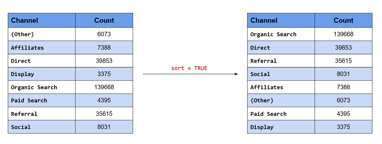
fct_count(channel, sort = TRUE)# A tibble: 8 × 2
f n
<fct> <int>
1 Organic Search 139668
2 Direct 39853
3 Referral 35615
4 Social 8031
5 Affiliates 7388
6 (Other) 6073
7 Paid Search 4395
8 Display 3375If you want to view the proportion along with the count, set the prop argument to TRUE.
fct_count(channel, prop = TRUE)# A tibble: 8 × 3
f n p
<fct> <int> <dbl>
1 (Other) 6073 0.0248
2 Affiliates 7388 0.0302
3 Direct 39853 0.163
4 Display 3375 0.0138
5 Organic Search 139668 0.571
6 Paid Search 4395 0.0180
7 Referral 35615 0.146
8 Social 8031 0.0329One of the important steps in data preparation/sanitization is to check if the levels are valid i.e. only levels which should be present in the data are actually present. fct_match() can be used to check validity of levels. It returns a logical vector if the level is present and an error if not.
channel |>
  fct_match("Social") |>
  table()
 FALSE   TRUE
236367   8031
16.1.2 Your Turn…
Display the count/frequency of the following variables in the descending order
devicelanding_pageexit_page
Check if
laptopis a level in thedevicecolumn.
16.1.3 Change Value of Levels
In this section, we will learn how to change the value of the levels. In order to keep it interesting, we will state an objective from our case study and then map it into a function from the forcats package.
Combine both Paid & Organic Search into a single level, Search
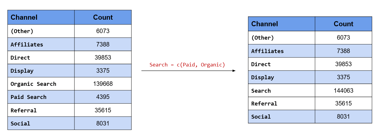
In this case, we want to change the value of two levels, Paid Search & Organic Search and give them the common value Search. You can also look at it as collapsing two levels into one. There are two functions we can use here:
fct_collapse()fct_recode()
Let us look at fct_collapse() first. After specifying the categorical variable, we specify the new value followed by a character vector of the existing values. Remember, the new value is not enclosed in quotes (single or double) but the existing values must be a character vector.
channel |>
  fct_collapse(Search = c("Paid Search", "Organic Search")) |>
  fct_count()
# A tibble: 7 × 2
f n
<fct> <int>
1 (Other) 6073
2 Affiliates 7388
3 Direct 39853
4 Display 3375
5 Search 144063
6 Referral 35615
7 Social 8031In the case of fct_recode(), each value being changed must be specified in a new line. Similar to fct_collapse(), the new value is not enclosed in quotes but the existing values must be.
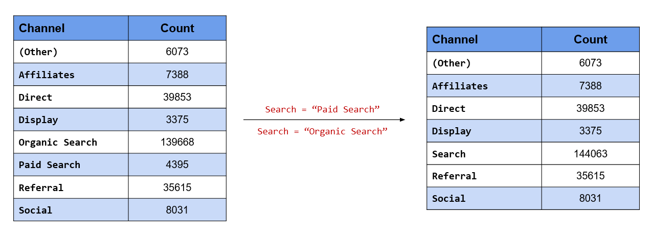
channel |>
  fct_recode(
    Search = "Paid Search",
    Search = "Organic Search"
  ) |>
  fct_count()
# A tibble: 7 × 2
f n
<fct> <int>
1 (Other) 6073
2 Affiliates 7388
3 Direct 39853
4 Display 3375
5 Search 144063
6 Referral 35615
7 Social 8031The dplyr and car packages also have recode functions.
Retain only those channels which have driven a minimum traffic of 5000 to the website
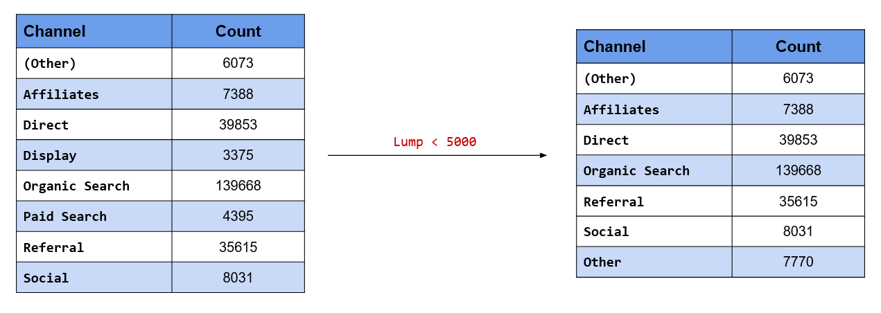
Instead of having all the channels, we desire to retain only those channels which have driven at least 5000 visits to the website. What about the rest of the channels which have driven less than 5000? We will recategorize them as Other. Keep in mind that we already have a (Other) level in our data. fct_lump_min() will lump together all levels which do not have a minimum count specified. In our case study, only Display drives less than 5000 visits and it will be categorized into Other.
channel |>
  fct_lump_min(min = 5000) |>
  fct_count()
# A tibble: 7 × 2
f n
<fct> <int>
1 (Other) 6073
2 Affiliates 7388
3 Direct 39853
4 Organic Search 139668
5 Referral 35615
6 Social 8031
7 Other 7770Retain only top 3 referring channels and categorize rest into Other
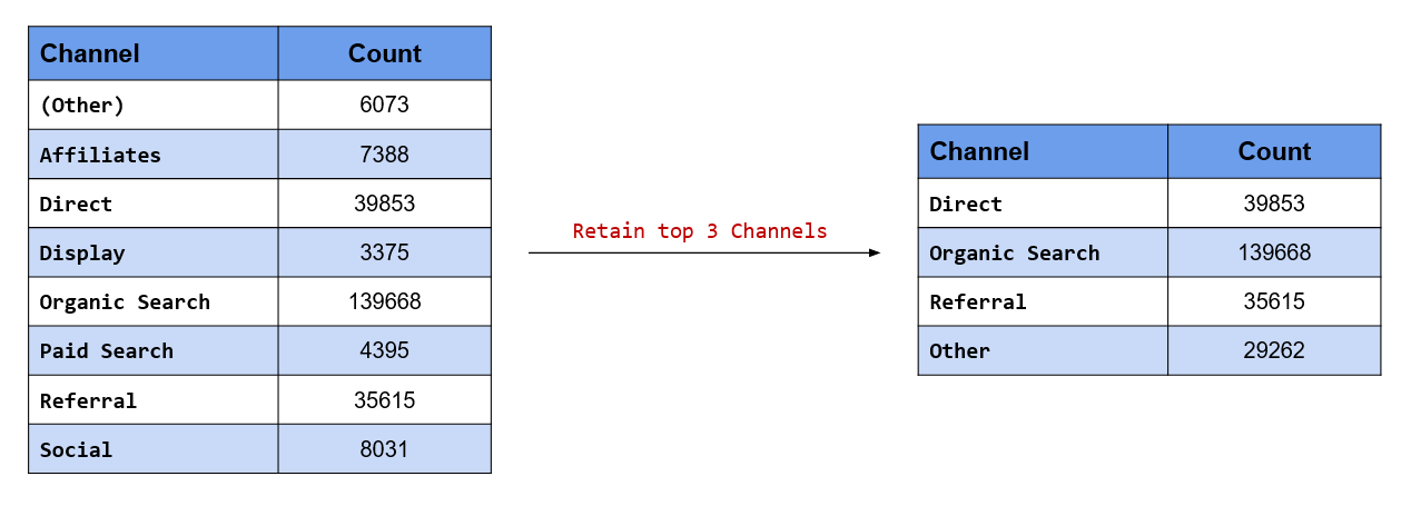
Suppose you decide to retain only the top 3 channels in terms of the traffic driven to the website. In our case study, these are Direct, Organic Search and Referral. We want to retain these 3 levels and categorize the rest as Other. fct_lump_n() will retain top n levels by count/frequency and lump the rest into Other.
channel |>
  fct_lump_n(n = 3) |>
  fct_count()
# A tibble: 4 × 2
f n
<fct> <int>
1 Direct 39853
2 Organic Search 139668
3 Referral 35615
4 Other 29262In our case, n is 3 and hence the top 3 channels in terms of traffic driven are retained while the rest are lumped into Other.
Retain only those channels which have driven at least 2% of the overall traffic
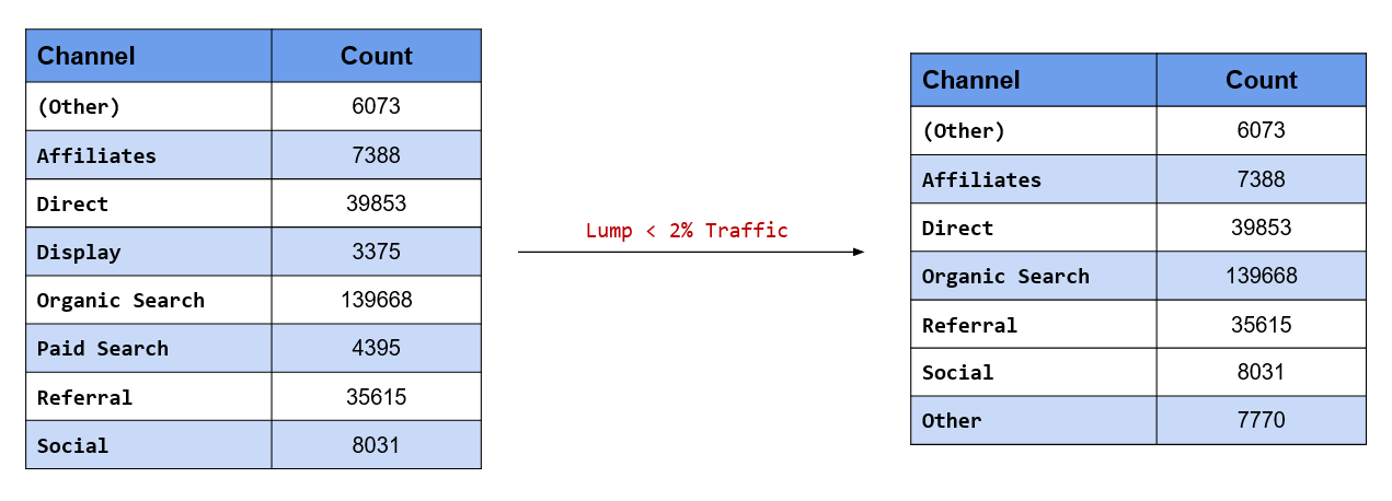
In the second scenario above, we retained channels based on minimum traffic driven by them to the website. The criteria was count of visits. If you want to specify the criteria as a percentage or proportion instead of count, use fct_lump_prop(). The criteria is a value between 0 and 1. In our case study, we want to retain channels that have driven at least 2% of the overall traffic. Hence, we have specified the criteria as 0.02.
channel |>
  fct_lump_prop(prop = 0.02) |>
  fct_count()
# A tibble: 7 × 2
f n
<fct> <int>
1 (Other) 6073
2 Affiliates 7388
3 Direct 39853
4 Organic Search 139668
5 Referral 35615
6 Social 8031
7 Other 7770As you can see, only Display drives less than 2% of overall traffic and has been lumped into Other.
Retain the following channels and merge the rest into Other
- Organic Search
- Direct
- Referral
In the previous scenarios, we have been retaining or lumping channels based on some criteria like count or percentage of traffic driven to the website. In this scenario, we want to retain certain levels by specifying their labels and combine the rest into Other. While we can use fct_collapse() or fct_recode(), a more appropriate function would be fct_other(). We will do a comparison of the three functions in a short while.
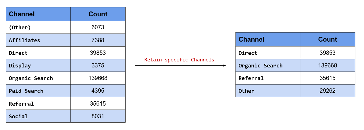
fct_other() has two arguments, keep and drop. keep is used when we know the levels we want to retain and drop is used when we know the levels we want to drop. In this scenario, we know the levels we want to retain and hence we will use the keep argument and specify them. Organic Search, Direct and Referral will be retained while the rest of the channels will be lumped into Other.
# channels to be retained
retain <- c("Organic Search", "Direct", "Referral")

channel |>
  fct_other(keep = retain) |> #<<
  fct_count()
# A tibble: 4 × 2
f n
<fct> <int>
1 Direct 39853
2 Organic Search 139668
3 Referral 35615
4 Other 29262Merge the following channels into Other and retain rest of them:
- Display
- Paid Search
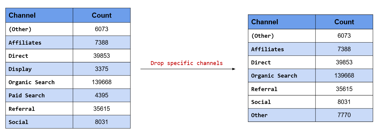
In this scenario, we know the levels we want to drop and hence we will use the drop argument and specify them. Display and Paid Search will be lumped into Other while the rest of the channels will be retained.
# channels to be dropped
dropped <- c("Display", "Paid Search")

channel |>
  fct_other(drop = dropped) |>
  fct_count()
# A tibble: 7 × 2
f n
<fct> <int>
1 (Other) 6073
2 Affiliates 7388
3 Direct 39853
4 Organic Search 139668
5 Referral 35615
6 Social 8031
7 Other 7770In the previous scenario, we said we will compare fct_other() with fct_collapse() and fct_recode(). Let us use the other two functions as well and see the difference.
# collapse
channel |>
  fct_collapse(Other = c("(Other)",
                         "Affiliates",
                         "Display",
                         "Paid Search",
                         "Social")) |>
  fct_count()
# A tibble: 4 × 2
f n
<fct> <int>
1 Other 29262
2 Direct 39853
3 Organic Search 139668
4 Referral 35615# recode
channel |>
fct_recode(Other = "(Other)",
Other = "Affiliates",
Other = "Display",
Other = "Paid Search",
Other = "Social") |>
fct_count()# A tibble: 4 × 2
f n
<fct> <int>
1 Other 29262
2 Direct 39853
3 Organic Search 139668
4 Referral 35615As you can observe, fct_other() requires less typing and is easier to specify.
Anonymize the data set before sharing it with your colleagues
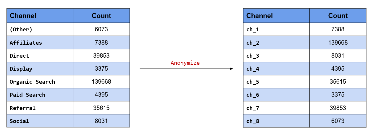
Anonymizing data is extremely important when you are sharing sensitive data with others. Here, we want to anonymize the channels which drive traffic to the website so that we can share it with others without divulging the names of the channels. fct_anon() allows us to anonymize the levels in the data. Using the prefix argument, we can specify the prefix to be used while anonymizing the data.
channel |>
  fct_anon(prefix = "ch_") |>
  fct_count()
# A tibble: 8 × 2
f n
<fct> <int>
1 ch_1 39853
2 ch_2 139668
3 ch_3 8031
4 ch_4 7388
5 ch_5 4395
6 ch_6 3375
7 ch_7 35615
8 ch_8 607316.1.4 Key Functions
| Function | Description |
|---|---|
| `fct_collapse()` | Collapse factor levels |
| `fct_recode()` | Recode factor levels |
| `fct_lump_min()` | Lump factor levels with count lesser than specified value |
| `fct_lump_n()` | Lump all levels except the top n levels |
| `fct_lump_prop()` | Lump factor levels with count lesser than specified proportion |
| `fct_lump_lowfreq()` | Lump together least frequent levels |
| `fct_other()` | Replace levels with Other level |
| `fct_anon()` | Anonymize factor levels |
16.1.5 Your Turn..
Combine the following levels in
landing_pageintoAccountMy AccountRegisterSign InYour Info
Combine levels in
landing_pagethat drive less than 1000 visits.Get top 10 landing and exit pages.
Get landing pages that drive at least 5% of the total traffic to the website.
Retain only the following levels in the
browsercolumn:ChromeFirefoxSafariEdge
Anonymize landing and exit page levels.
16.1.6 Add / Remove Levels
In this small section, we will learn to:
- add new levels
- drop levels
- make missing values explicit
Add a new level, Blog
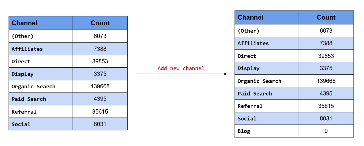
fct_expand() allows us to add new levels to the data. The label of the new level must be specified after the variable name and must be enclosed in quotes. If the level already exists, it will be ignored. Let us add a new level, Blog.
channel |>
  fct_expand("Blog") |> #<<
  levels()
[1] "(Other)" "Affiliates" "Direct" "Display"
[5] "Organic Search" "Paid Search" "Referral" "Social"
[9] "Blog" Drop existing level
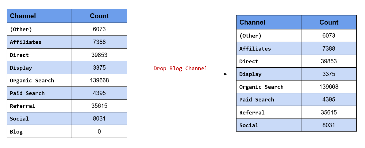
On the other hand, fct_drop() will drop levels which have no values i.e. unused levels. If you want to drop only specific levels, use the only argument and specify the name of the level in quotes. Let us drop the new level we added in the previous example.
channel |>
  fct_expand("Blog") |>
  fct_drop() |> #<<
  levels()
[1] "(Other)" "Affiliates" "Direct" "Display"
[5] "Organic Search" "Paid Search" "Referral" "Social" Make missing values explicit

In our data set, the gender column has many missing values, and in R, missing values are represented by NA. Suppose you are sharing the data or analysis with someone who is not an R user, and does not know what NA represents. In such a scenario, we can use the fct_na_value_to_level() function to make the missing values in the gender column explicit i.e. it will appear as (Missing) instead of NA. This will help non R users to understand that there are missing values in the data.
data |>
  pull(gender) |>
  fct_na_value_to_level(level = "(Missing)") |>  #<<
  fct_count()
# A tibble: 3 × 2
f n
<fct> <int>
1 female 40565
2 male 61617
3 (Missing) 14221616.1.7 Key Functions
| Function | Description |
|---|---|
| `fct_expand()` | Add additional levels to a factor |
| `fct_drop()` | Drop unused factor levels |
| `fct_na_value_to_level()` | Make missing values explicit |
16.1.8 Change Order of Levels
In this last part of this section, we will learn how to change the order of the levels. We will look at the following scenarios from our case study:
We want to make
- Organic Search the first level
- Referral the third level
- Display the last level
Organic Search is the first level
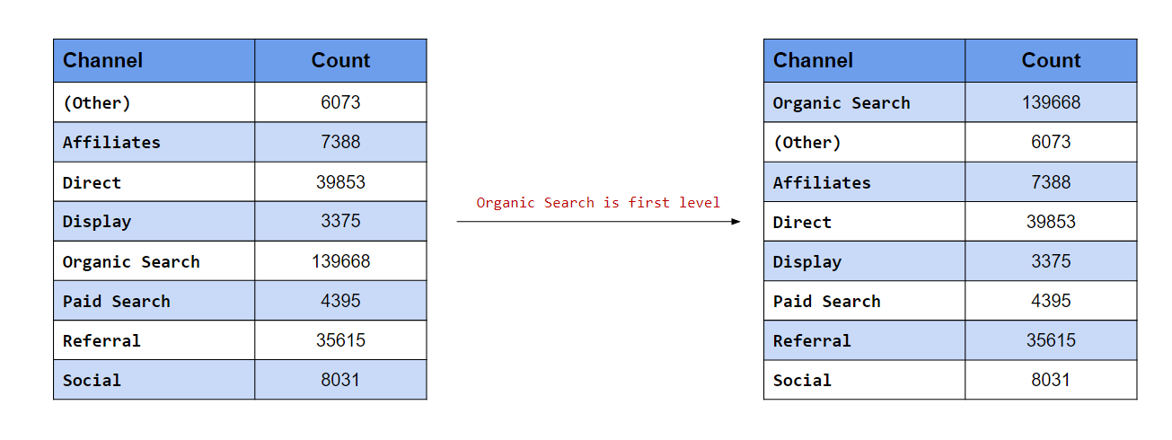
In this scenario, we want the levels to appear in a certain order. In the first case, we want Organic Search to be the first level. fct_relevel() allows us to manually reorder the levels. To move a level to the beginning, specify the label (it must be enclosed in quotes).
levels(channel)[1] "(Other)" "Affiliates" "Direct" "Display"
[5] "Organic Search" "Paid Search" "Referral" "Social" channel |>
fct_relevel("Organic Search") |> #<<
levels()[1] "Organic Search" "(Other)" "Affiliates" "Direct"
[5] "Display" "Paid Search" "Referral" "Social" Referral is the third level
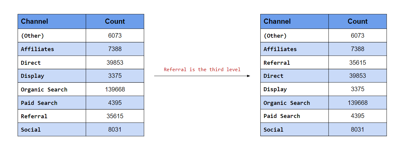
The after argument is useful when we want to move the level to the end or anywhere between the beginning and end. In the second case, we want Referral to be the third level. After specifying the label, use the after argument and specify the level after which Referral should appear. Since we want to move it to the third position, we will set the value of after to 2 i.e. Referral should come after the second position.
levels(channel)[1] "(Other)" "Affiliates" "Direct" "Display"
[5] "Organic Search" "Paid Search" "Referral" "Social" channel |>
fct_relevel("Referral", after = 2) |> #<<
levels()[1] "(Other)" "Affiliates" "Referral" "Direct"
[5] "Display" "Organic Search" "Paid Search" "Social" Display is the last level
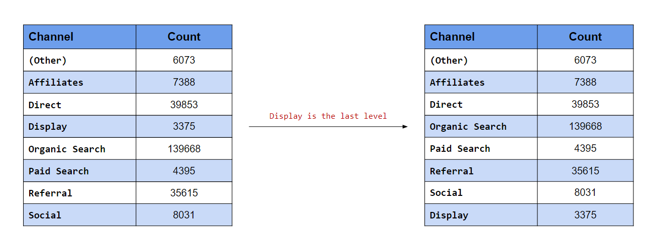
In this last case, we want to move Display to the end. If you know the number of levels, you can specify a value here. In our data, there are eight channels i.e. eight levels, so we can set the value of after to 7. What happens when we do not know the number of levels or if they tend to vary? In such cases, to move a level to the end, set the value of after to Inf.
levels(channel)[1] "(Other)" "Affiliates" "Direct" "Display"
[5] "Organic Search" "Paid Search" "Referral" "Social" channel |>
fct_relevel("Display", after = Inf) |> #<<
levels()[1] "(Other)" "Affiliates" "Direct" "Organic Search"
[5] "Paid Search" "Referral" "Social" "Display" Let us now look at a scenario where we want to order the levels by
- frequency (largest to smallest)
- order of appearance (in data)
Order levels by frequency
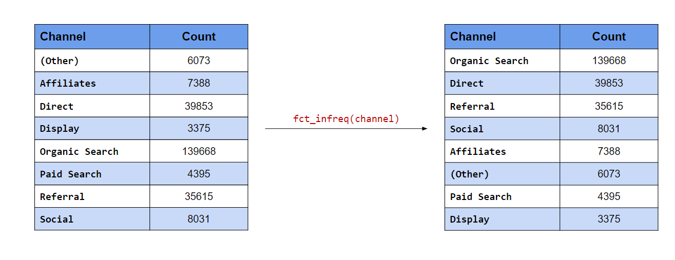
In the first case, the levels with the most frequency should appear at the top. fct_infreq() will order the levels by their frequency.
levels(channel)[1] "(Other)" "Affiliates" "Direct" "Display"
[5] "Organic Search" "Paid Search" "Referral" "Social" # order levels by frequency
channel |>
fct_infreq() |> #<<
levels()[1] "Organic Search" "Direct" "Referral" "Social"
[5] "Affiliates" "(Other)" "Paid Search" "Display" Order levels by appearance
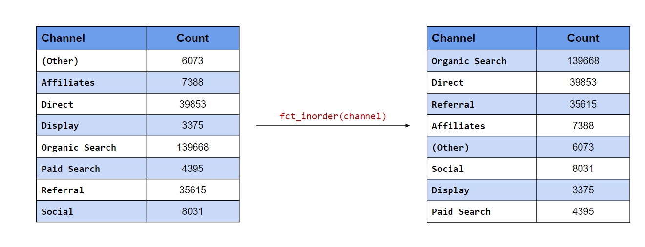
In the second case, the order of the levels should be the same as the order of their appearance in the data. fct_inorder() will order the levels according to the order in which they appear in the data.
levels(channel)[1] "(Other)" "Affiliates" "Direct" "Display"
[5] "Organic Search" "Paid Search" "Referral" "Social" # order levels in order of appearance
channel |>
fct_inorder() |> #<<
levels()[1] "Organic Search" "Direct" "Referral" "Affiliates"
[5] "(Other)" "Social" "Display" "Paid Search" Reverse the order of the levels
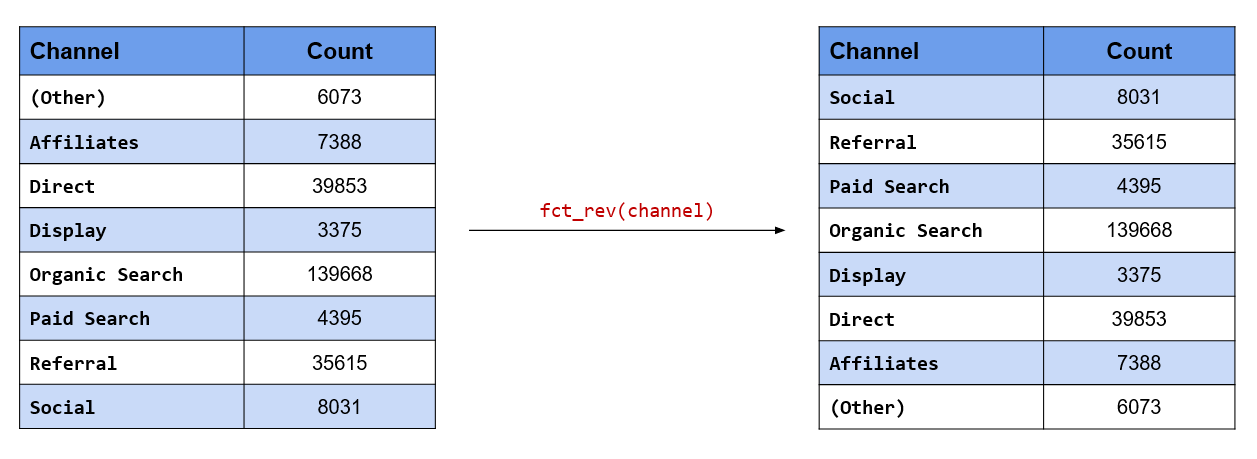
The order of the levels can be reversed using fct_rev().
levels(channel)[1] "(Other)" "Affiliates" "Direct" "Display"
[5] "Organic Search" "Paid Search" "Referral" "Social" # reverse order of levels
channel |>
fct_rev() |> #<<
levels()[1] "Social" "Referral" "Paid Search" "Organic Search"
[5] "Display" "Direct" "Affiliates" "(Other)" Randomly shuffle the order of the levels
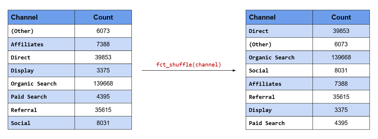
The order of the levels can be randomly shuffled using fct_shuffle().
levels(channel)[1] "(Other)" "Affiliates" "Direct" "Display"
[5] "Organic Search" "Paid Search" "Referral" "Social" # randomly shuffle order of levels
channel |>
fct_shuffle() |> #<<
levels()[1] "Organic Search" "Social" "(Other)" "Referral"
[5] "Display" "Paid Search" "Direct" "Affiliates" 16.1.9 Key Functions
| Function | Description |
|---|---|
| `fct_relevel()` | Reorder factor levels |
| `fct_shift()` | Shift factor levels |
| `fct_infreq()` | Reorder factor levels by frequency |
| `fct_rev()` | Reverse order of factor levels |
| `fct_inorder()` | Reorder factor levels by first appearance |
| `fct_shuffle()` | Randomly shuffle factor levels |
16.1.10 Your Turn…
Make
Homefirst level in thelanding_pagecolumn.Make
Apparelsecond level in thelanding_pagecolumn.Make
Specialslast level in thelanding_pagecolumn.Order the levels in the browser by frequency:
Order the levels in landing page by appearance:
Shuffle the levels in os
Reverse the levels in browser
16.2 Data Visualization
16.2.1 Introduction
In this section, we will learn to visualize categorical data. We will look at the following type of plots:
- univariate bar plot
- bivariate bar plot
- grouped
- stacked
- proportional
- mosaic plot
- pie chart
- donut chart
We will be using ggplot2 in this chapter. So you should know the basics of data visualization with ggplot2. If you are new or have never used ggplot2, do not worry. We have several tutorials and an ebook on ggplot2, you can go through them first and then come back to this section.
16.2.2 Bar Plot
Bar charts provide a visual representation of categorical data. The bars can be plotted either vertically or horizontally. The categories/groups appear along the horizontal X axis and the height of the bar represents a measured value.
ggplot(data) +
  geom_bar(aes(x = device), fill = "blue") +
  xlab("Device") + ylab("Count")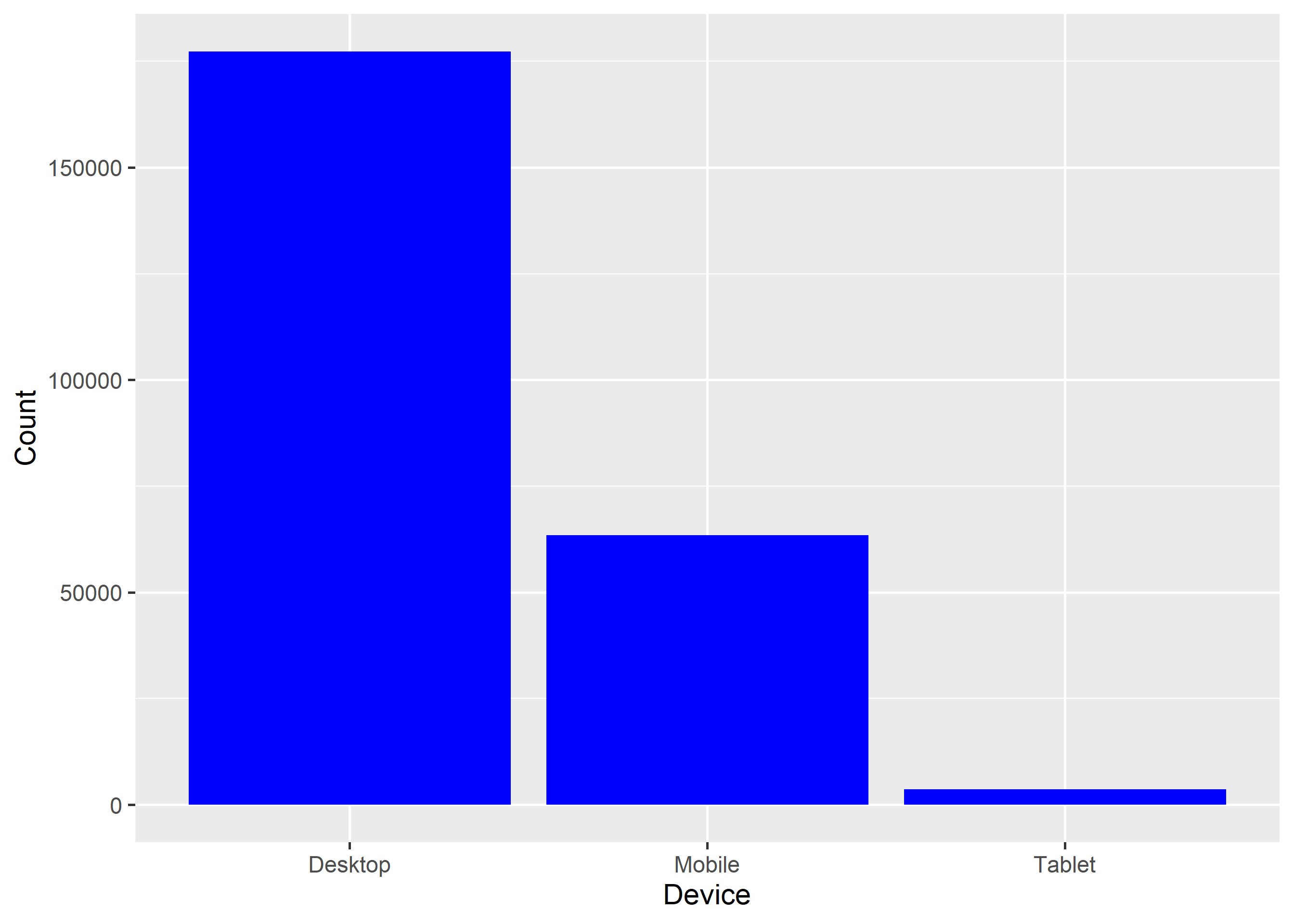
In the above example, the bars represent the count/frequency of the categories. If the bars represent continuous data, the value could be mean or sum of the variable being represented.
16.2.3 Grouped Bar Plot
A grouped bar chart plots values for two levels of a categorical variable instead of one. You should use grouped bar chart when making comparisons across different categories of data. Use it when you want to look at how the second category variable changes within each level of the first and vice versa.
ggplot(data) +
  geom_bar(aes(x = device, fill = gender), position = "dodge") +
  xlab("Device") + ylab("Count")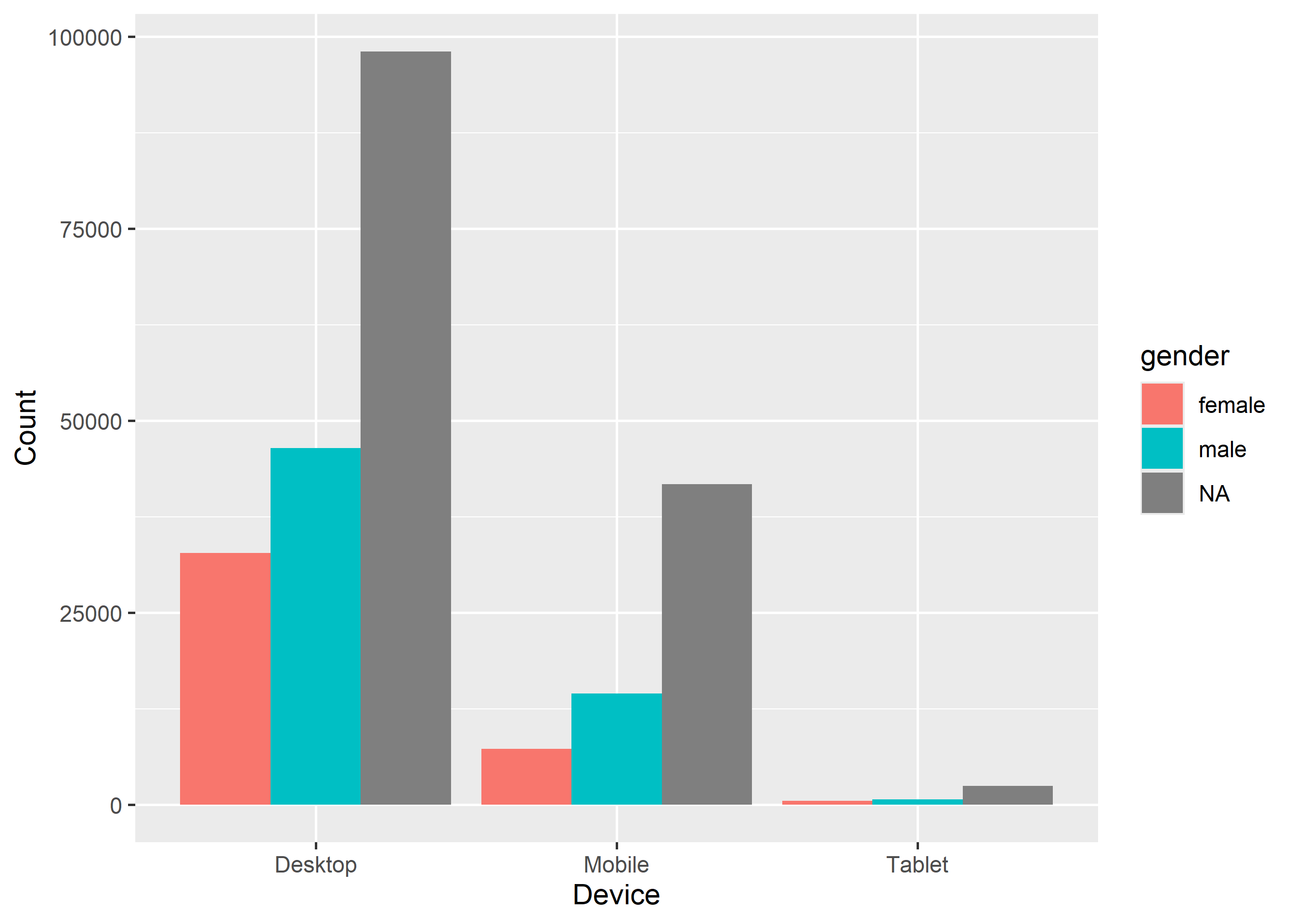
16.2.4 Stacked Bar Plot
In stacked bar plots, the bars are stacked on top of each other instead of placing them next to each other. Use stacked bar plots while looking at cumulative value.
ggplot(data) +
  geom_bar(aes(x = device, fill = gender)) +
  xlab("Device") + ylab("Count")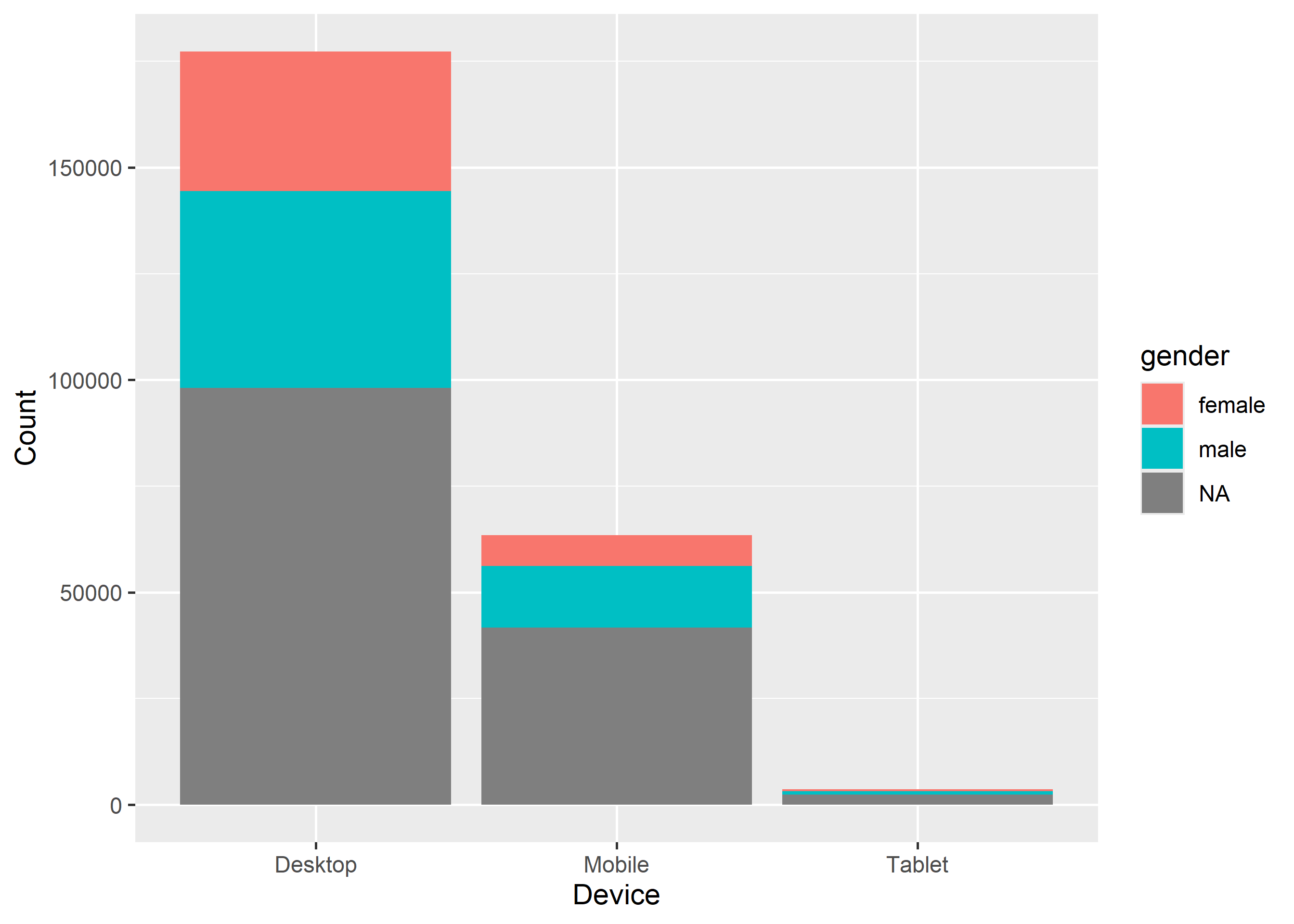
16.2.5 Proportional Bar Plot
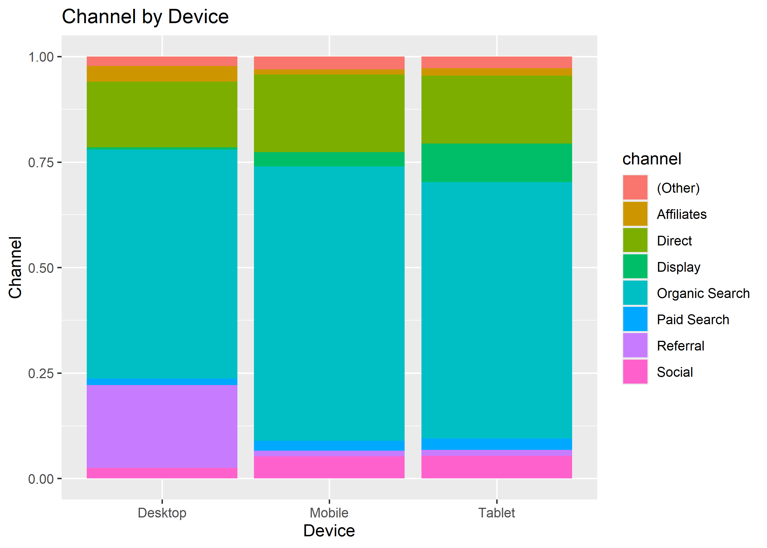
Also known as percent stacked plot, the height of all bars in this plot are the same. The distribution of the second categorical variable is scaled to 1 or 100. The length of each bar is determined by its share in the category. Use this when you want to concurrently observe each of several variables as they fluctuate and as their percentage ratio’s change.
data |>
  select(device, gender) |>
  table() |>
  tibble::as_tibble() |>
  ggplot(aes(x = device, y = n, fill = gender)) +
  geom_bar(stat = "identity", position = "fill") +
  xlab("Device") + ylab("Gender")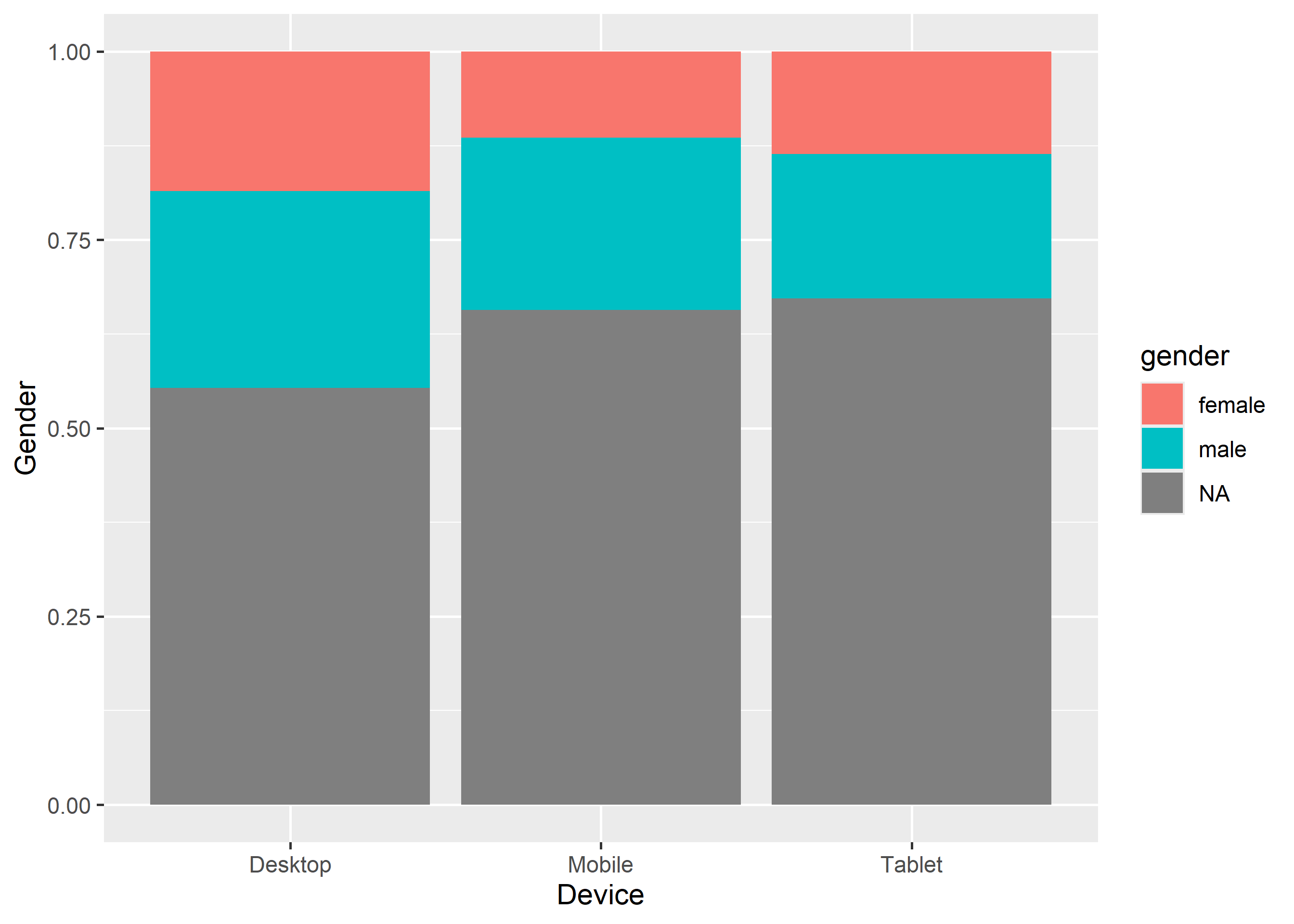
16.2.6 Mosaic Plot
A mosaic plot is a graphical representation of a two way table or contingency table. It was introduced by Hartigan & Kleiner and is divided into rectangles. Proportions on horizontal axis represents the number of observations for each level of the X variable. The vertical length of each rectangle is proportional to the proportion of Y variable in each level of X variable.
Mosaic plots need the ggmosaic package (archived on CRAN) and are out of scope here — they are covered in the ggplot2 ebook.
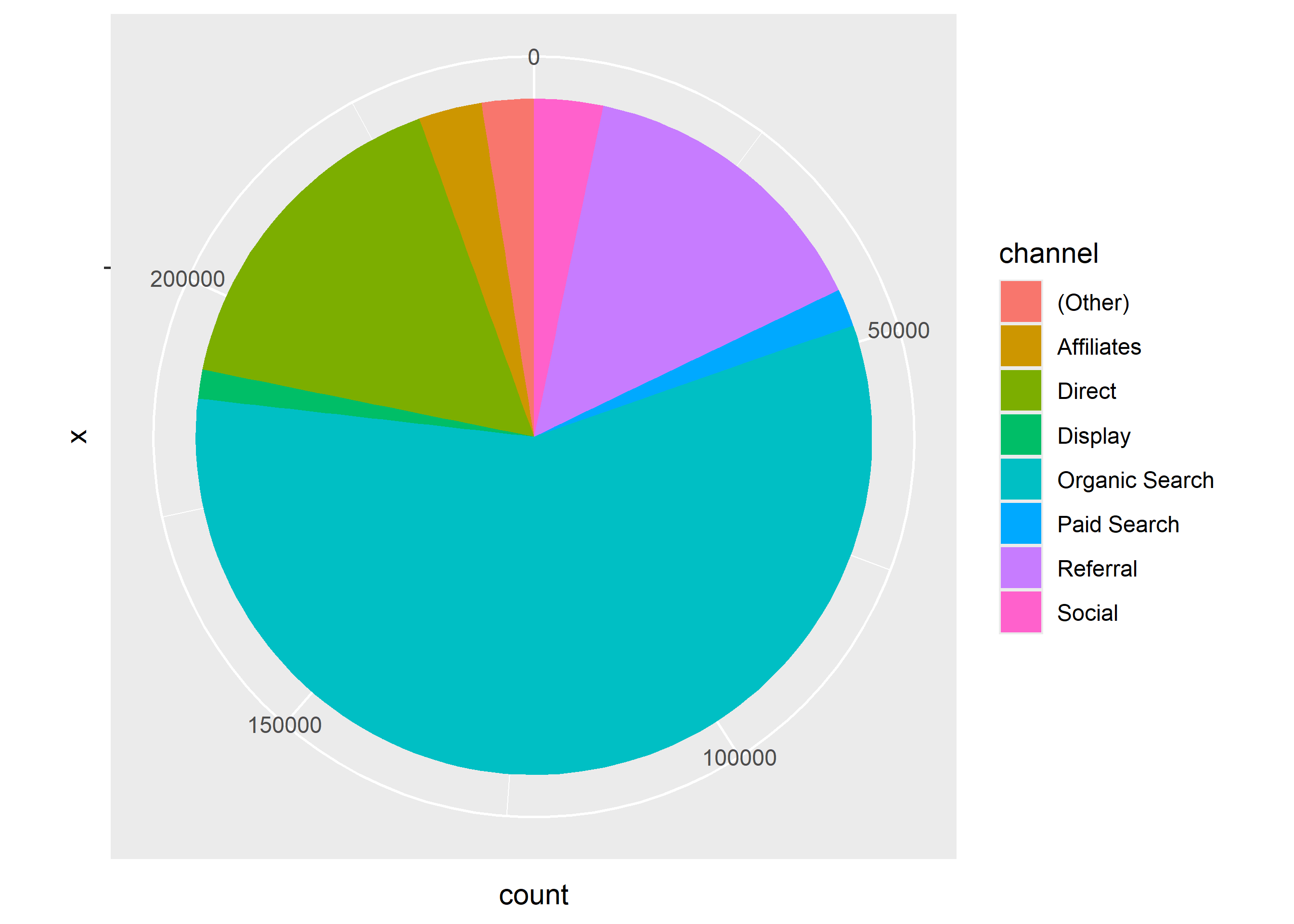
16.2.7 Pie Chart
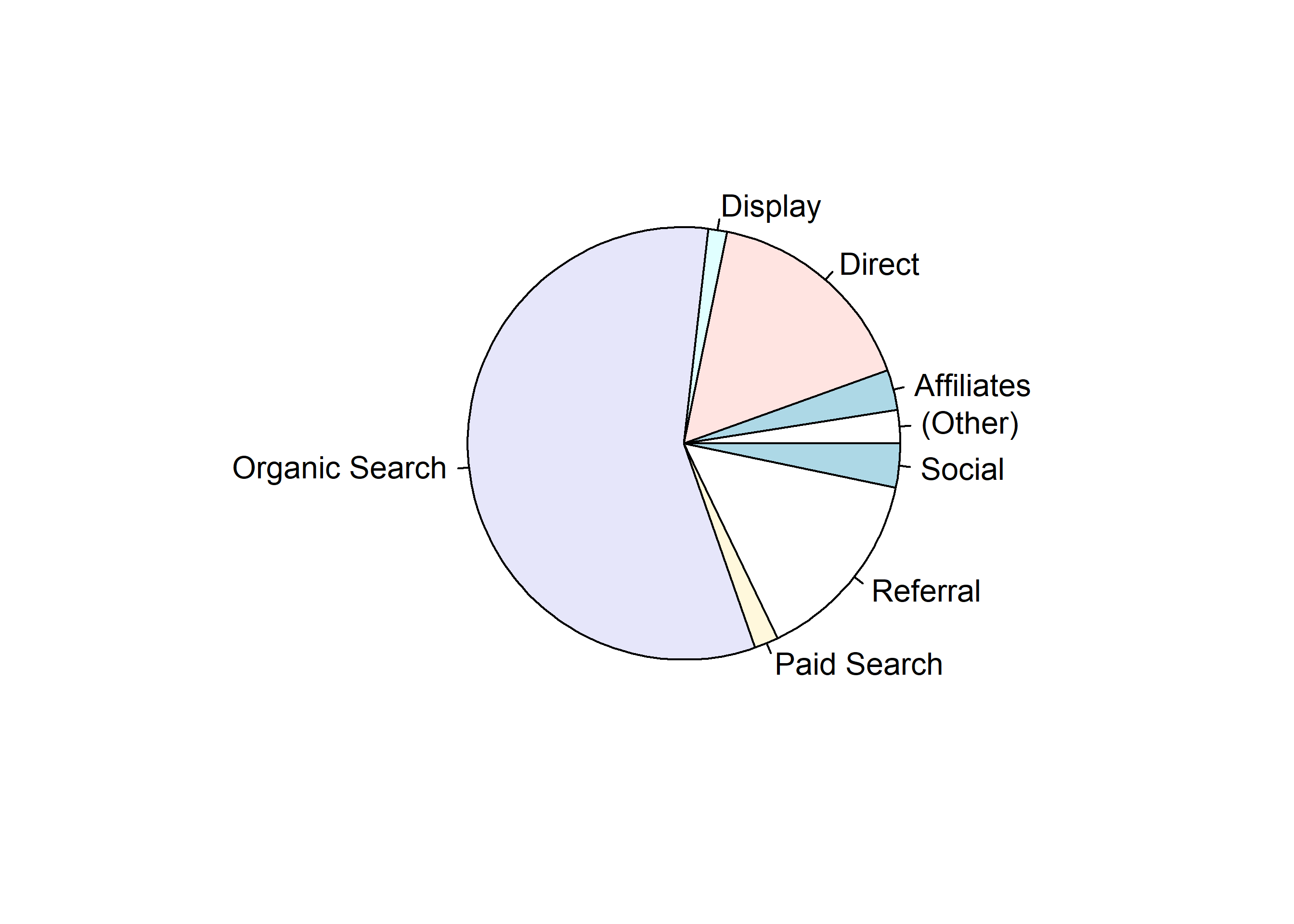
Pie chart is a circular chart, divided into slices to show relevant sizes of data. It shows the distribution of the different levels of a categorical variable as a circle is divided into radial slices. Each level corresponds with a single slice of the circle and size indicates the proportion of the level. Use it when comparing each group’s contribution to the whole as opposed to comparing groups to each other.
Base R
data |>
  pull(device) |>
  table() |>
  pie()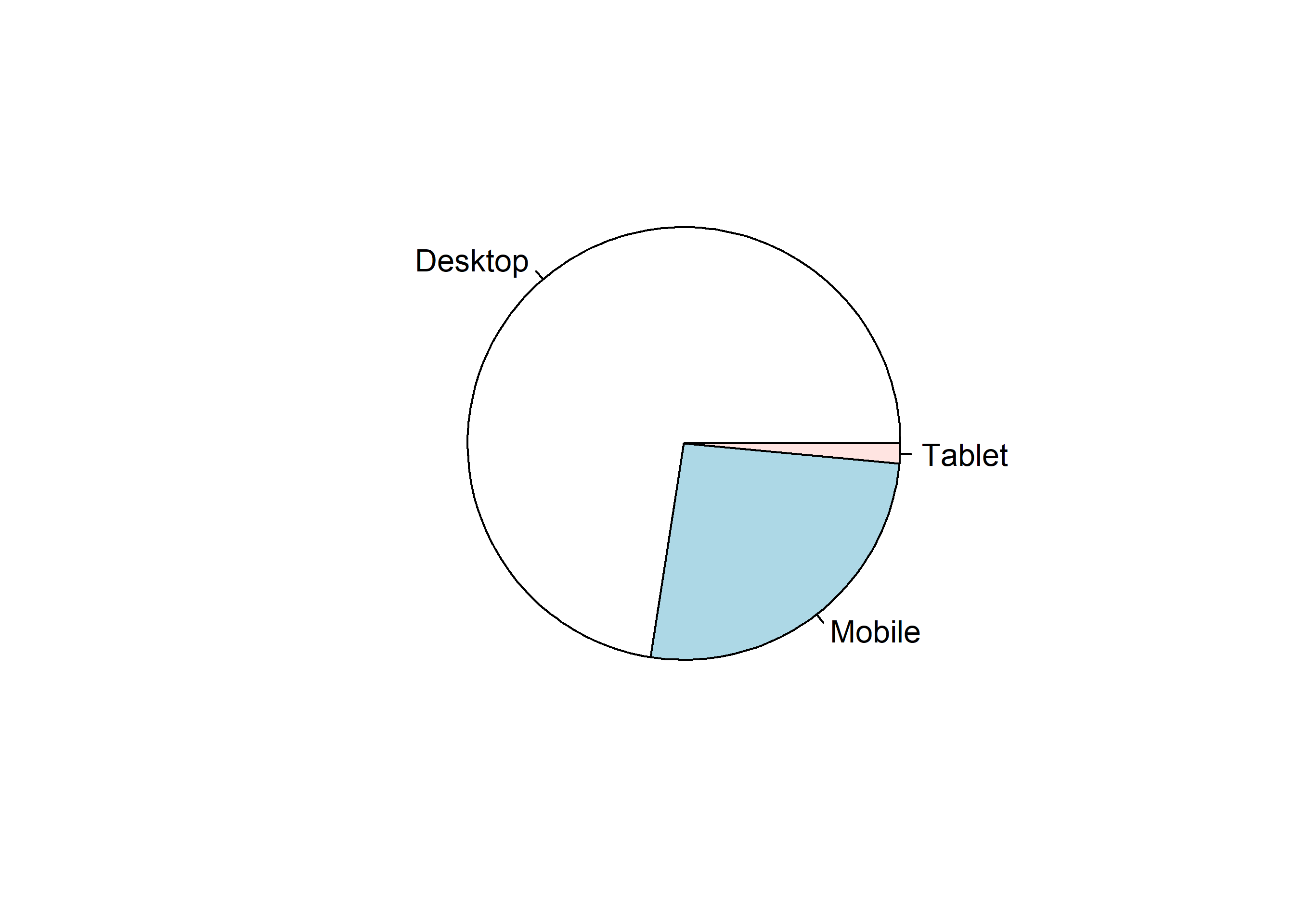
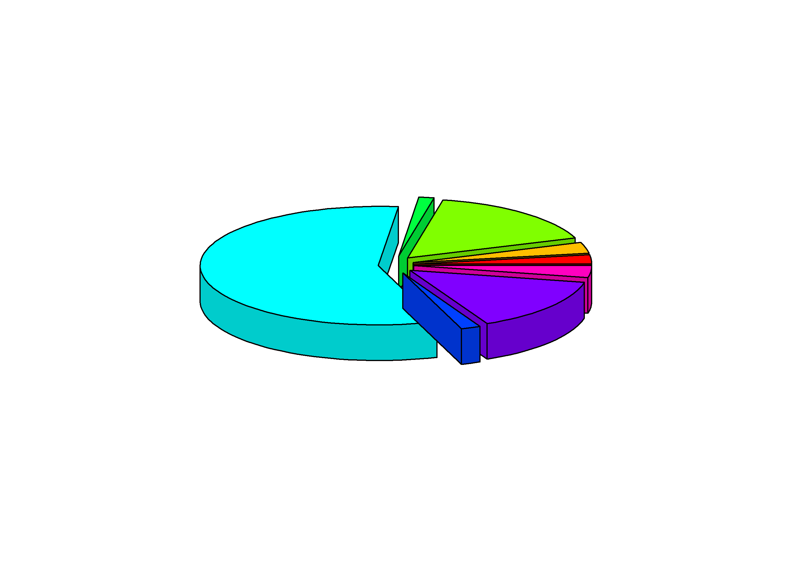
3D Pie Chart
data |>
  pull(device) |>
  table() |>
  pie3D(explode = 0.1)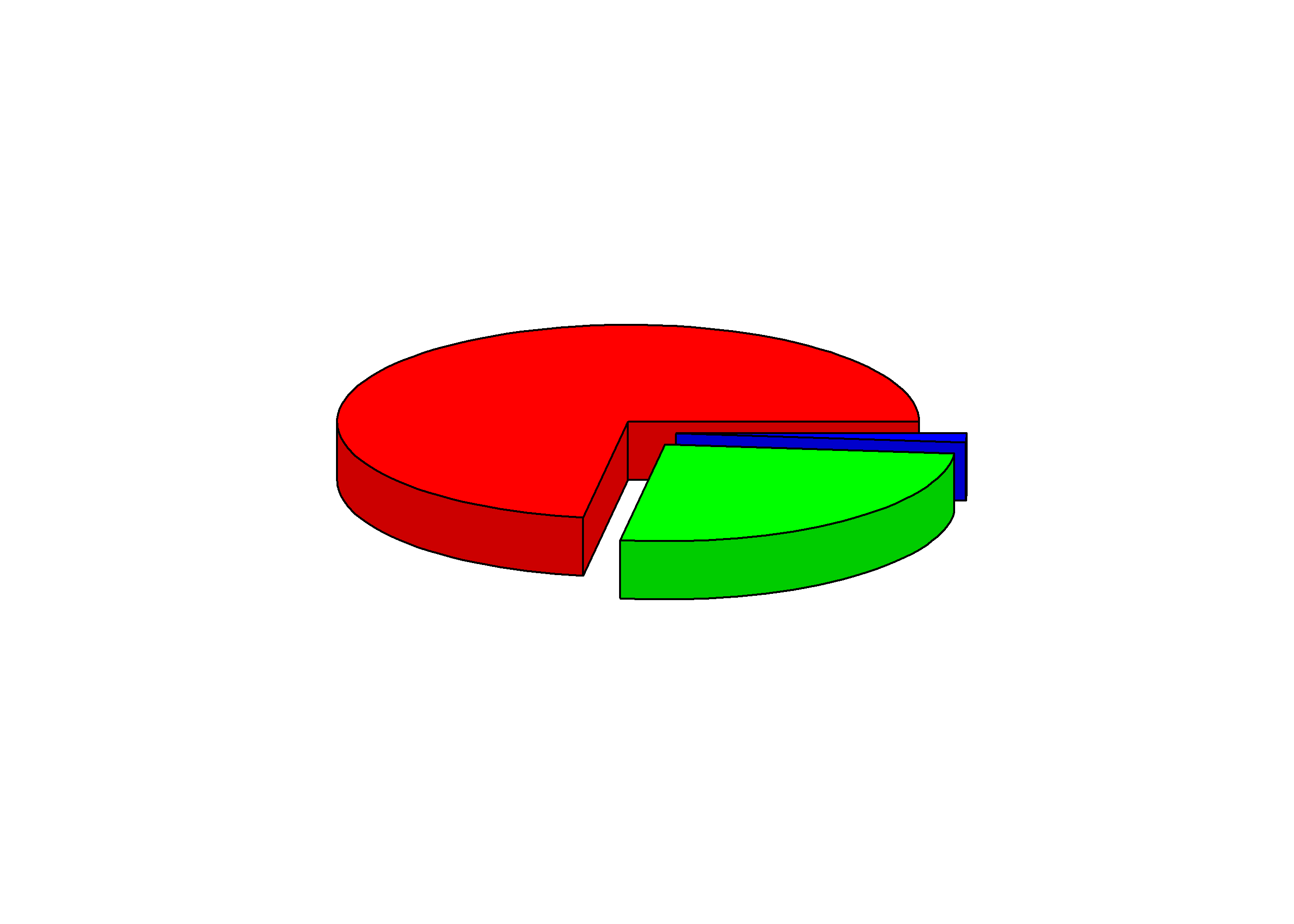
ggplot2
data |>
  pull(device) |>
  fct_count() |>
  rename(device = f, count = n) |>
  ggplot() +
  geom_bar(aes(x = "", y = count, fill = device), width = 1, stat = "identity") +
  coord_polar("y", start = 0)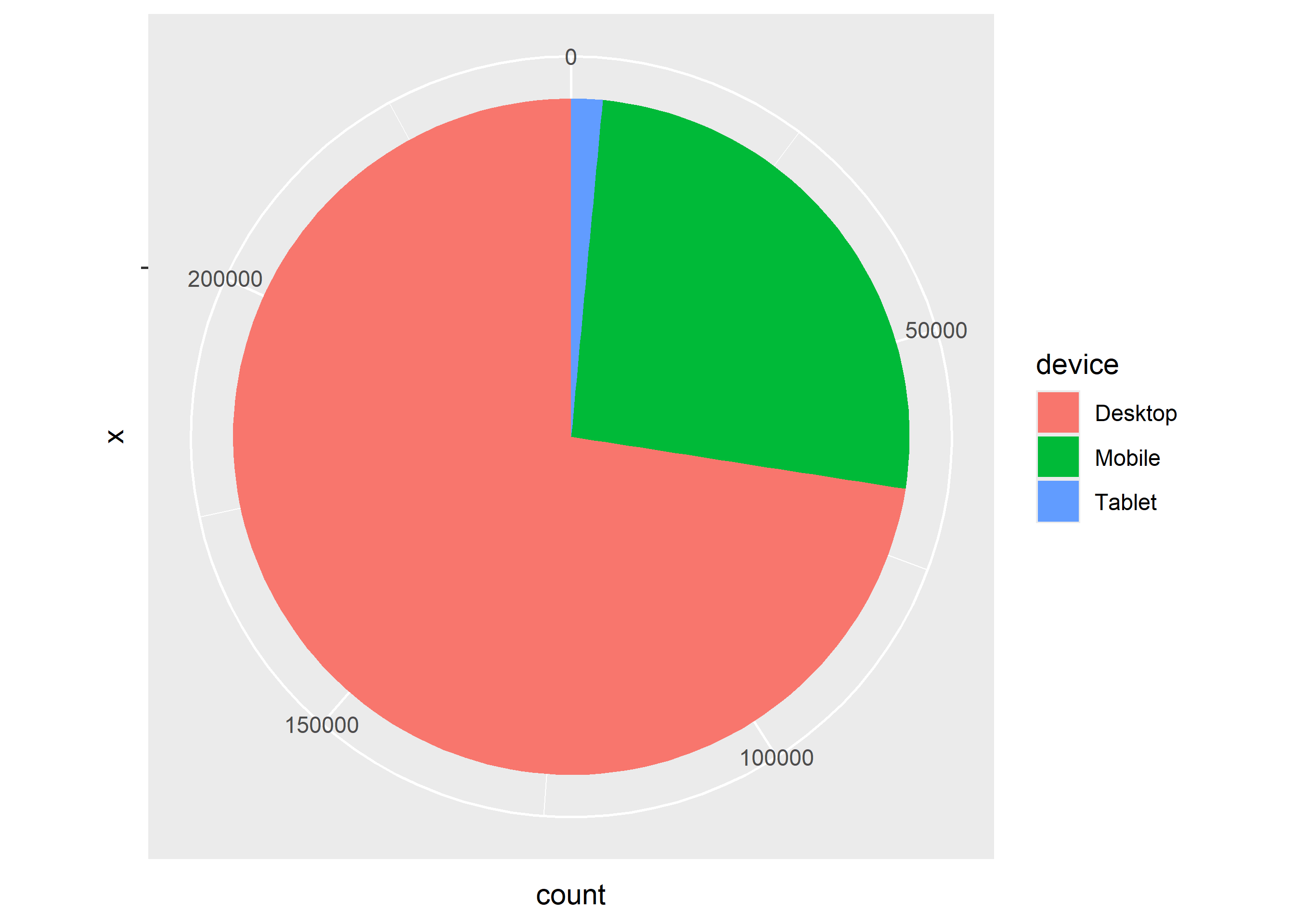
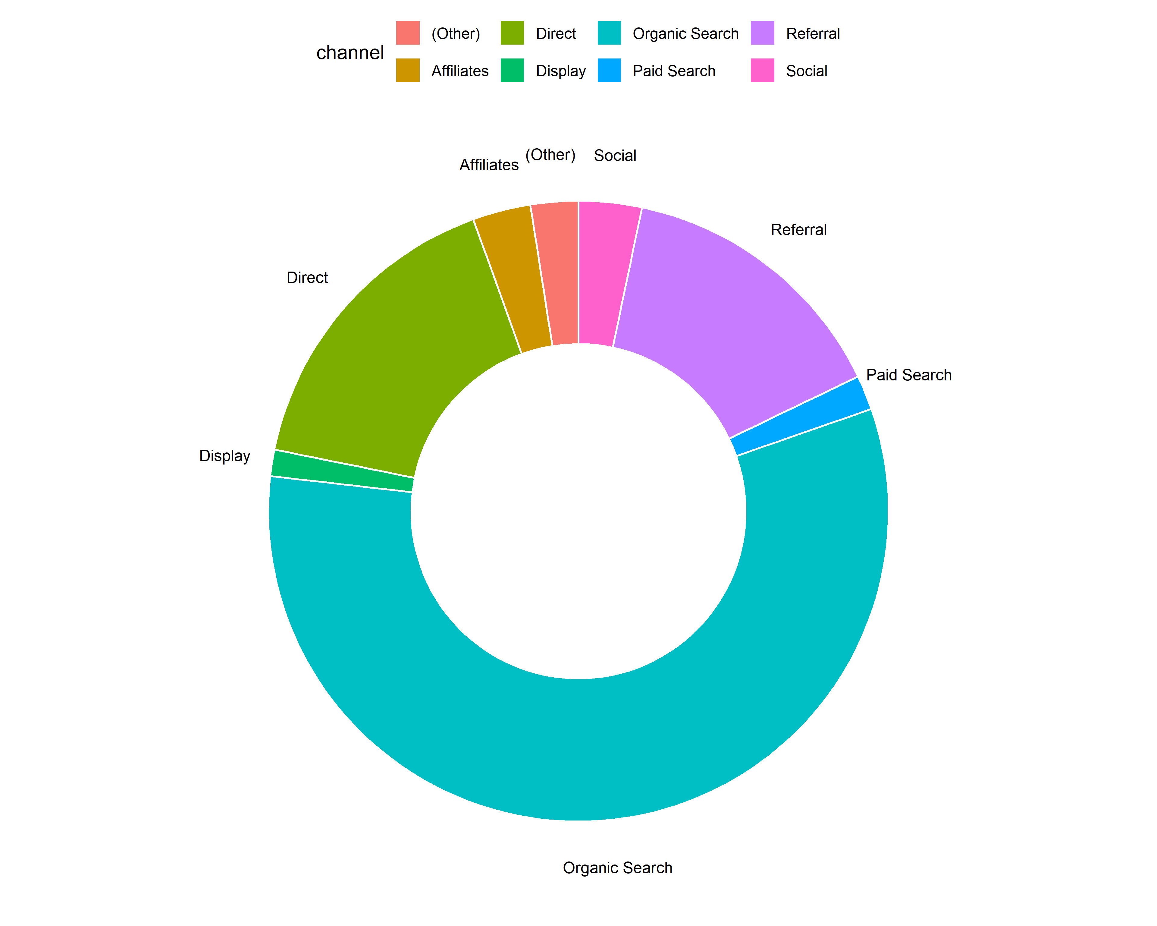
16.2.8 Donut Chart
Donut chart is a variation of the pie chart. It has a round hole in the middle which makes it look like a donut. The focus is on the length of the arcs and not the proportions of the slices. Blank spaces inside donut chart can be used to display information inside it.
data |>
  pull(device) |>
  fct_count() |>
  rename(device = f, count = n) |>
  ggdonutchart("count", label = "device", fill = "device", color = "white",
               palette = c("#00AFBB", "#E7B800", "#FC4E07"))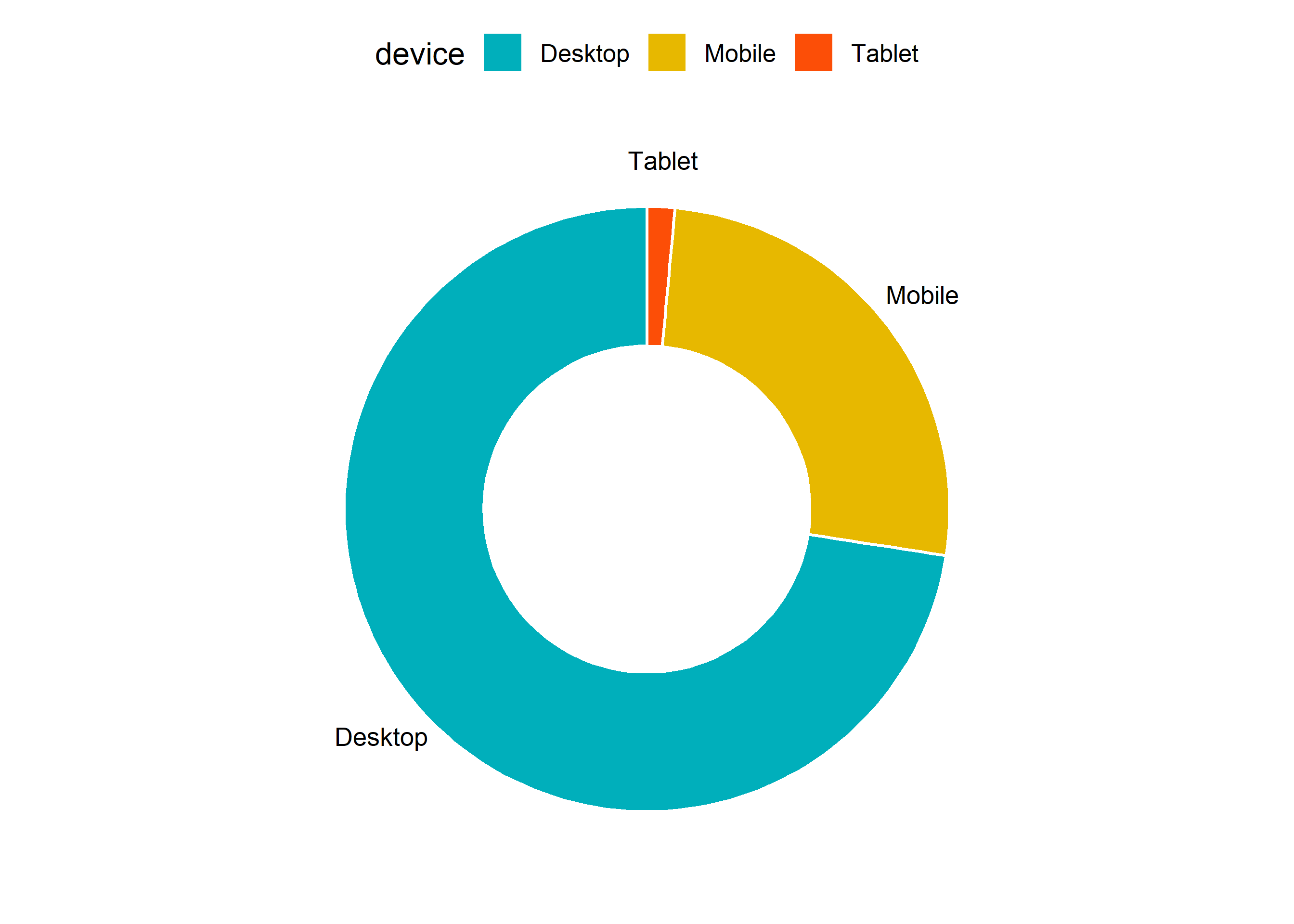
16.2.9 Summary
- Bar charts provide a visual representation of categorical data.
- Use grouped bar chart to make comparison against different categories of data.
- Use stacked bar chart while looking at cumulative data.
- Use proportional bar chart when you want to concurrently observe each of the several variables as they fluctuate.
- Use mosaic plot to discover associations between two variables.
- Use pie chart and donut chart when comparing each group’s contribution to the whole.
16.2.10 Your Turn…
Generate all the below plots:
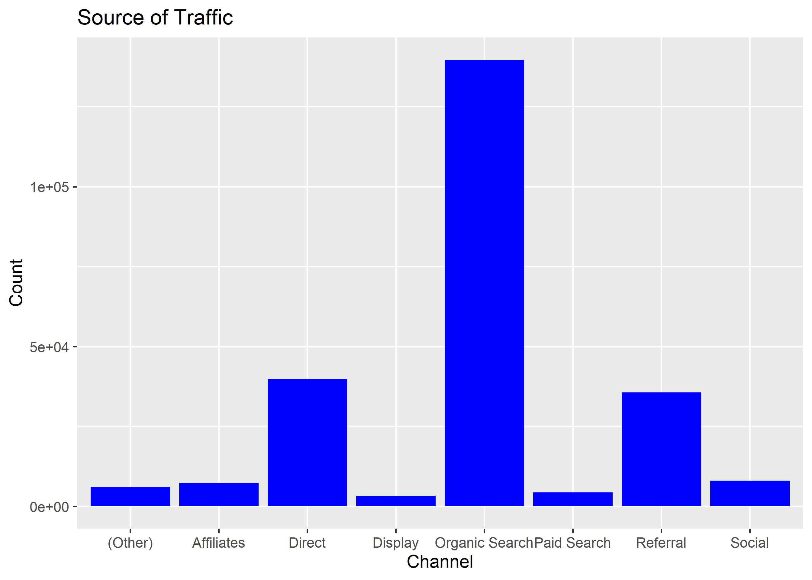
- Bar plot of
channel
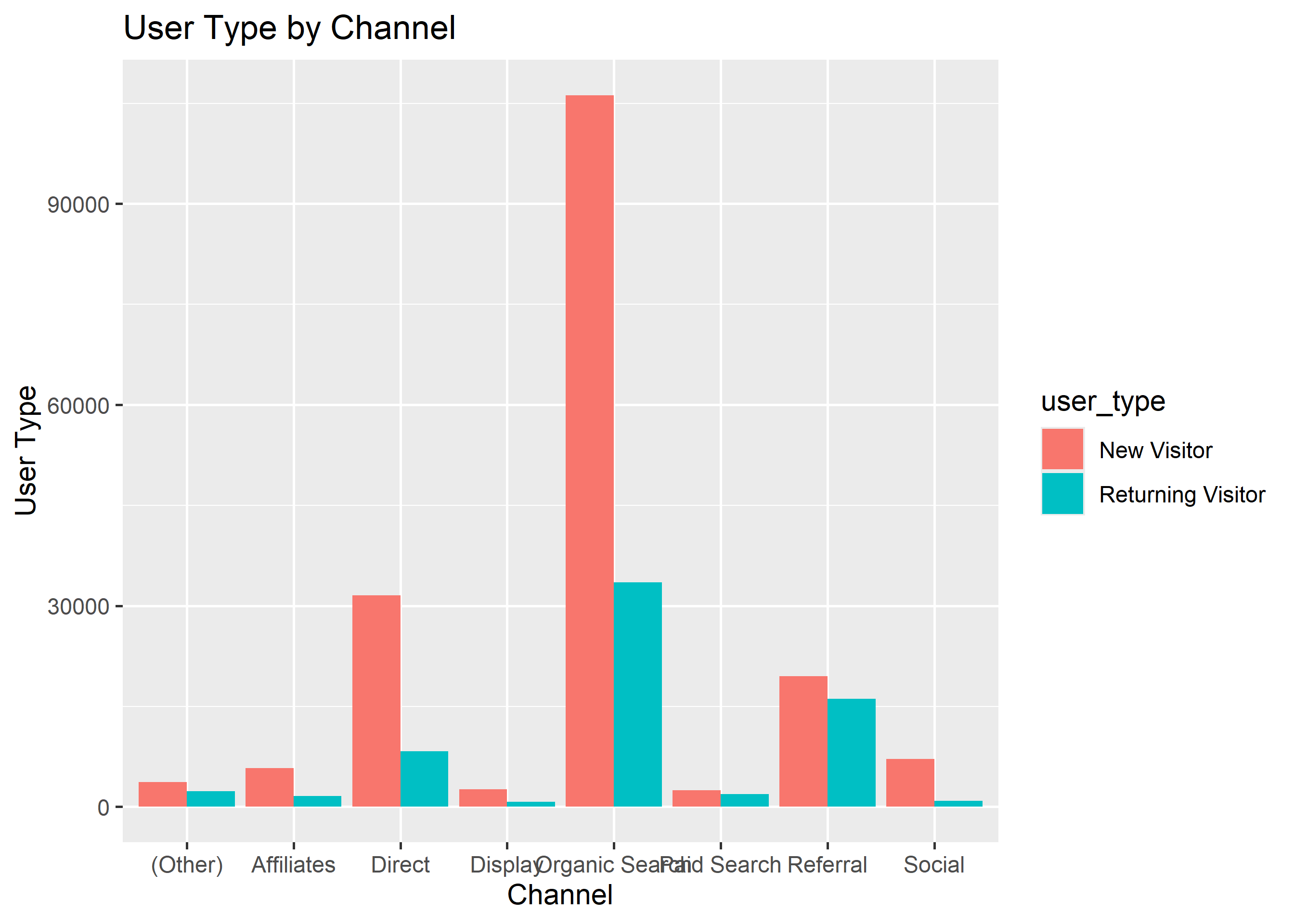
- Display grouped bar plot of
user_typebychannel
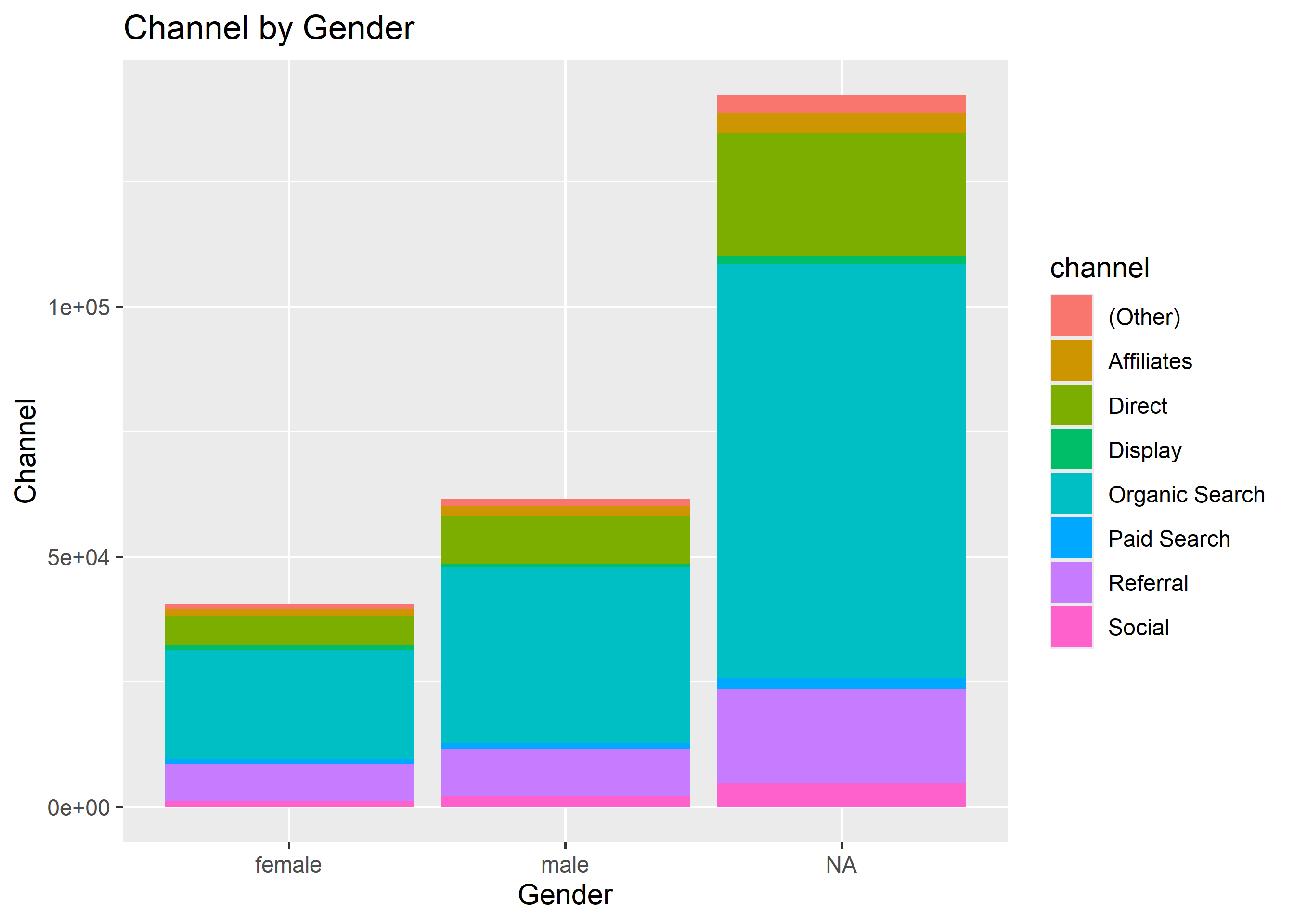
- Display stacked bar plot of
channelbygender
- Display proportional bar plot of
channelbydevice
- Display mosaic plot of
devicebychannel
Mosaic plots need the ggmosaic package (archived on CRAN) and are out of scope here — they are covered in the ggplot2 ebook.
- Display pie or donut chart of
channel
6.1 Pie Chart
6.2 3D Pie Chart
6.3 Pie Chart (ggplot2)
6.4 Donut Chart
16.3 Useful R Packages
Below are a list of functions from different R pacakges for summarizing categorical data.
16.3.1 Summarize Variables
Hmisc::describe(data$device)data$device
n missing distinct
244398 0 3
Value Desktop Mobile Tablet
Frequency 177282 63482 3634
Proportion 0.725 0.260 0.015janitor::tabyl(data$device) data$device n percent
Desktop 177282 0.72538237
Mobile 63482 0.25974844
Tablet 3634 0.01486919epiDisplay::tab1(data$device)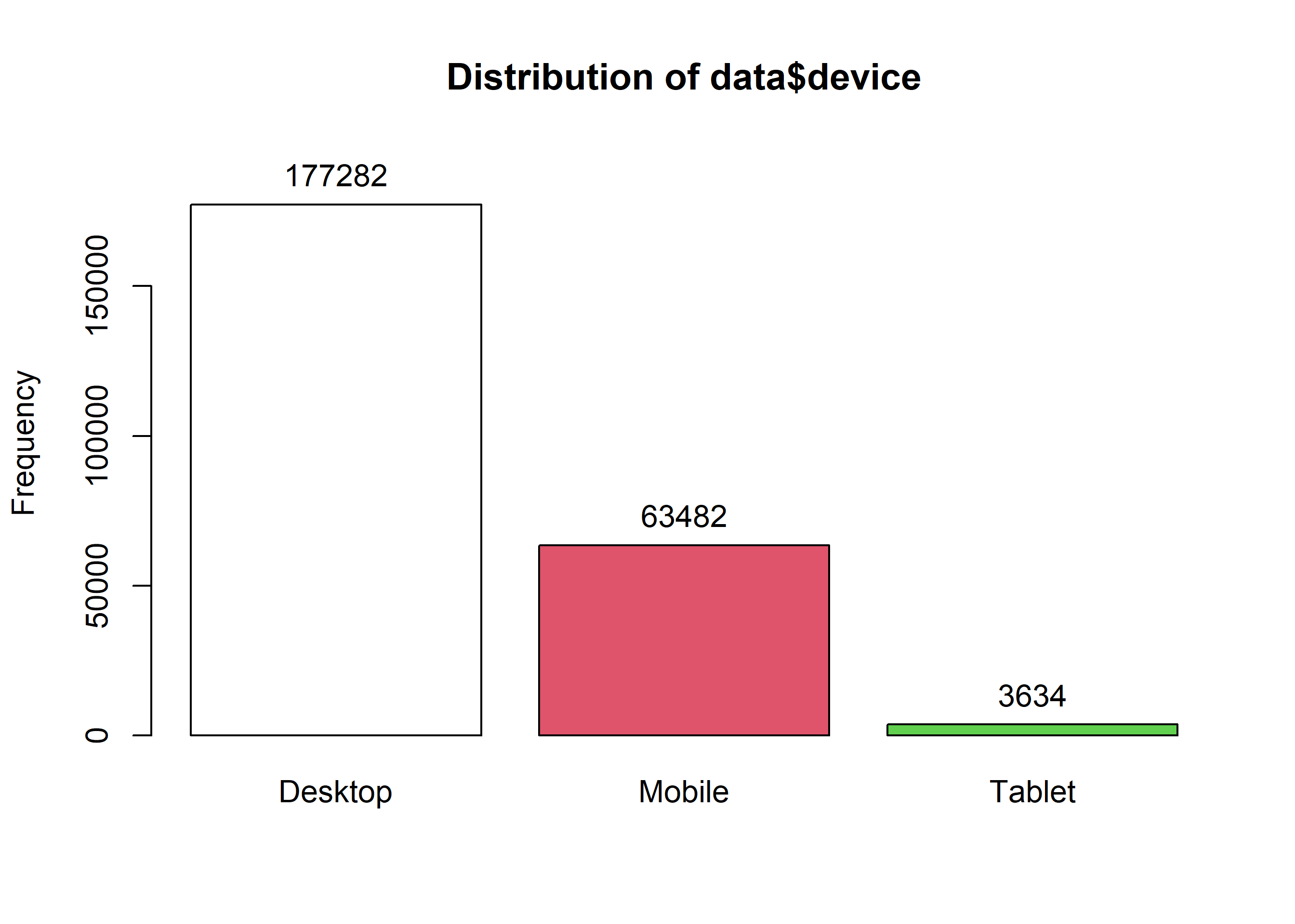
data$device :
        Frequency Percent Cum. percent
Desktop    177282    72.5         72.5
Mobile      63482    26.0         98.5
Tablet       3634     1.5        100.0
Total 244398 100.0 100.0summarytools::freq(data$device)Frequencies
data$device
Type: Factor
Freq % Valid % Valid Cum. % Total % Total Cum.
------------- -------- --------- -------------- --------- --------------
Desktop 177282 72.54 72.54 72.54 72.54
Mobile 63482 25.97 98.51 25.97 98.51
Tablet 3634 1.49 100.00 1.49 100.00
<NA> 0 0.00 100.00
Total 244398 100.00 100.00 100.00 100.00questionr::freq(data$device) n % val%
Desktop 177282 72.5 72.5
Mobile 63482 26.0 26.0
Tablet 3634 1.5 1.5descriptr::ds_freq_table(data, device) Variable: device
-----------------------------------------------------------------------
Levels Frequency Cum Frequency Percent Cum Percent
-----------------------------------------------------------------------
Desktop 177282 177282 72.54 72.54
-----------------------------------------------------------------------
Mobile 63482 240764 25.97 98.51
-----------------------------------------------------------------------
Tablet 3634 244398 1.49 100
-----------------------------------------------------------------------
Total 244398 - 100.00 -
-----------------------------------------------------------------------16.3.2 Summarize Data Set
minilytics <- select(data, device, browser, os)
psych::describe(minilytics)
vars n mean sd median trimmed mad min max range skew kurtosis
device* 1 244398 1.29 0.49 1 1.22 0.0 1 3 2 1.31 0.58
browser* 2 244398 8.22 4.84 6 7.14 0.0 1 26 25 1.80 1.43
os* 3 244398 8.80 4.47 8 8.99 8.9 1 16 15 -0.08 -1.36
se
device* 0.00
browser* 0.01
os* 0.01skimr::skim(minilytics)| Name | minilytics |
| Number of rows | 244398 |
| Number of columns | 3 |
| _______________________ | |
| Column type frequency: | |
| factor | 3 |
| ________________________ | |
| Group variables | None |
Variable type: factor
| skim_variable | n_missing | complete_rate | ordered | n_unique | top_counts |
|---|---|---|---|---|---|
| device | 0 | 1 | FALSE | 3 | Des: 177282, Mob: 63482, Tab: 3634 |
| browser | 0 | 1 | FALSE | 26 | Chr: 192176, Saf: 35323, Fir: 6420, Edg: 3787 |
| os | 0 | 1 | FALSE | 16 | Win: 91223, Mac: 66171, And: 39055, iOS: 27866 |
summarytools::dfSummary(minilytics)Data Frame Summary
minilytics
Dimensions: 244398 x 3
Duplicates: 244317
-----------------------------------------------------------------------------------------------------
No Variable Stats / Values Freqs (% of Valid) Graph Valid Missing
---- ---------- ----------------------- -------------------- ------------------- ---------- ---------
1 device 1. Desktop 177282 (72.5%) IIIIIIIIIIIIII 244398 0
[factor] 2. Mobile 63482 (26.0%) IIIII (100.0%) (0.0%)
3. Tablet 3634 ( 1.5%)
2 browser 1. Amazon Silk 168 ( 0.1%) 244398 0
[factor] 2. Android Browser 101 ( 0.0%) (100.0%) (0.0%)
3. Android Webview 1215 ( 0.5%)
4. APKPure 1 ( 0.0%)
5. BlackBerry 7 ( 0.0%)
6. Chrome 192176 (78.6%) IIIIIIIIIIIIIII
7. Coc Coc 45 ( 0.0%)
8. Edge 3787 ( 1.5%)
9. Firefox 6420 ( 2.6%)
10. Internet Explorer 700 ( 0.3%)
[ 16 others ] 39778 (16.3%) III
3 os 1. (not set) 179 ( 0.1%) 244398 0
[factor] 2. Android 39055 (16.0%) III (100.0%) (0.0%)
3. BlackBerry 16 ( 0.0%)
4. Chrome OS 14038 ( 5.7%) I
5. Firefox OS 4 ( 0.0%)
6. iOS 27866 (11.4%) II
7. Linux 5781 ( 2.4%)
8. Macintosh 66171 (27.1%) IIIII
9. OS/2 3 ( 0.0%)
10. Playstation 4 15 ( 0.0%)
[ 6 others ] 91270 (37.3%) IIIIIII
-----------------------------------------------------------------------------------------------------tableone::CreateTableOne(vars = c("device", "os"), data = minilytics)
                      Overall
  n                   244398
  device (%)
     Desktop          177282 (72.5)
     Mobile            63482 (26.0)
     Tablet             3634 ( 1.5)
  os (%)
     (not set)           179 ( 0.1)
     Android           39055 (16.0)
     BlackBerry           16 ( 0.0)
     Chrome OS         14038 ( 5.7)
     Firefox OS            4 ( 0.0)
     iOS               27866 (11.4)
     Linux              5781 ( 2.4)
     Macintosh         66171 (27.1)
     OS/2                  3 ( 0.0)
     Playstation 4        15 ( 0.0)
     Playstation Vita      1 ( 0.0)
     Samsung               5 ( 0.0)
     Tizen                20 ( 0.0)
     Windows           91223 (37.3)
     Windows Phone        13 ( 0.0)
Xbox 8 ( 0.0) desctable::desctable(minilytics) N %
1 device 244398 NA
2 device: Desktop 177282 7.253824e+01
3 device: Mobile 63482 2.597484e+01
4 device: Tablet 3634 1.486919e+00
5 browser 244398 NA
6 browser: Amazon Silk 168 6.874033e-02
7 browser: Android Browser 101 4.132603e-02
8 browser: Android Webview 1215 4.971399e-01
9 browser: APKPure 1 4.091687e-04
10 browser: BlackBerry 7 2.864181e-03
11 browser: Chrome 192176 7.863239e+01
12 browser: Coc Coc 45 1.841259e-02
13 browser: Edge 3787 1.549522e+00
14 browser: Firefox 6420 2.626863e+00
15 browser: Internet Explorer 700 2.864181e-01
16 browser: Maxthon 5 2.045843e-03
17 browser: Mozilla Compatible Agent 13 5.319192e-03
18 browser: MRCHROME 1 4.091687e-04
19 browser: Opera 1145 4.684981e-01
20 browser: Opera Mini 52 2.127677e-02
21 browser: Playstation 4 15 6.137530e-03
22 browser: Playstation Vita Browser 1 4.091687e-04
23 browser: Puffin 18 7.365036e-03
24 browser: Safari 35323 1.445306e+01
25 browser: Safari (in-app) 658 2.692330e-01
26 browser: Samsung Internet 2065 8.449333e-01
27 browser: SeaMonkey 3 1.227506e-03
28 browser: Seznam 1 4.091687e-04
29 browser: UC Browser 174 7.119535e-02
30 browser: User-Agent:Mozilla 28 1.145672e-02
31 browser: YaBrowser 276 1.129305e-01
32 os 244398 NA
33 os: (not set) 179 7.324119e-02
34 os: Android 39055 1.598008e+01
35 os: BlackBerry 16 6.546698e-03
36 os: Chrome OS 14038 5.743910e+00
37 os: Firefox OS 4 1.636675e-03
38 os: iOS 27866 1.140189e+01
39 os: Linux 5781 2.365404e+00
40 os: Macintosh 66171 2.707510e+01
41 os: OS/2 3 1.227506e-03
42 os: Playstation 4 15 6.137530e-03
43 os: Playstation Vita 1 4.091687e-04
44 os: Samsung 5 2.045843e-03
45 os: Tizen 20 8.183373e-03
46 os: Windows 91223 3.732559e+01
47 os: Windows Phone 13 5.319192e-03
48 os: Xbox 8 3.273349e-03Try it live
TipTry it in your browser
Edit the code below and press Run. It executes entirely in your browser via WebR — no R installation needed. The runtime downloads once, on this page only.